Readings:
Numpy/Scipy References
Can you add a scalar to a vector? Explain why or why not.
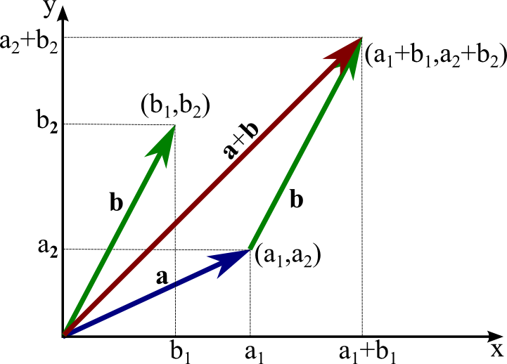
Consider vectors describing distance travelled in 2D.
Make two functions:
add two vectors.
Make it work for any number of dimensions
If we have two vectors: ${\bf{x}} = \begin{bmatrix} x_1 \\x_2 \\ \vdots \\ x_k \end{bmatrix}$ and ${\bf{y}} = \begin{bmatrix} y_1 \\y_2 \\ \vdots \\ y_k \end{bmatrix}$
The dot product is written: ${\bf{x}} \cdot {\bf{y}} = x_{1}y_{1}+x_{2}y_{2}+\cdots+x_{k}y_{k}$
If $\mathbf{x} \cdot \mathbf{y} = 0$ then $x$ and $y$ are orthogonal
What is $\mathbf{x} \cdot \mathbf{x}$?
Choose appropriate data structures for your vectors
Make it work for any number of dimensions
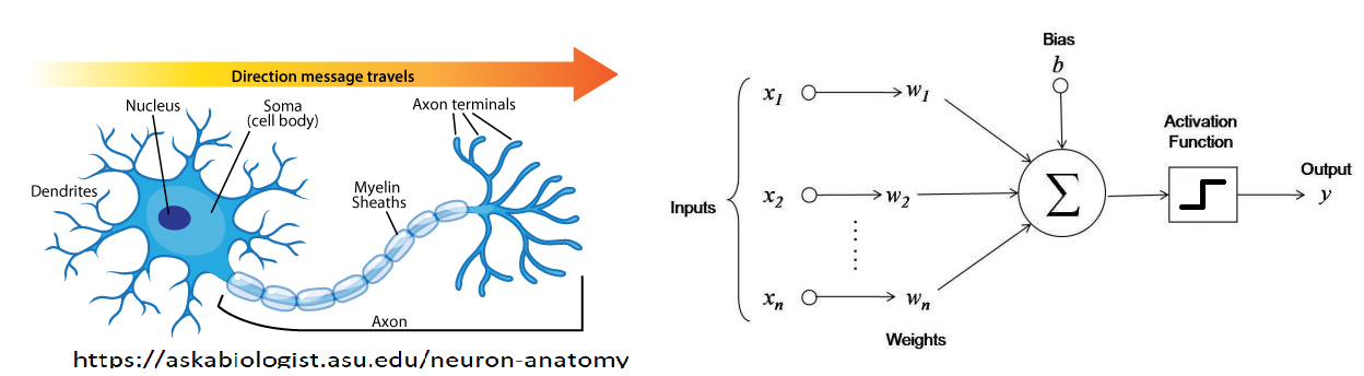
Use your dot product function to make an artificial neuron function $f(\mathbf x) = y$
Use the signum function for the activation function.
You may heard modern AI is based on matrix multiplication... this is because matrix multiplication consists of multiple dot products in parallel
Make a class for "dense" vectors that contains all your functions thus far.
Add dunder support for addition, scalar multiplication. What other possibilities might there be?
Put your class in a separate file in the path so you can import it and use the class.
You have created a starting point for your own homwmade numpy module.
View numpy as library of efficient vector functions.

All modern AI tools and much of Data Science tools is based on "drop-in replacements" of numpy. Basically the same basic programming syntax, but coded to run efficiently on GPUs or large server arrays.
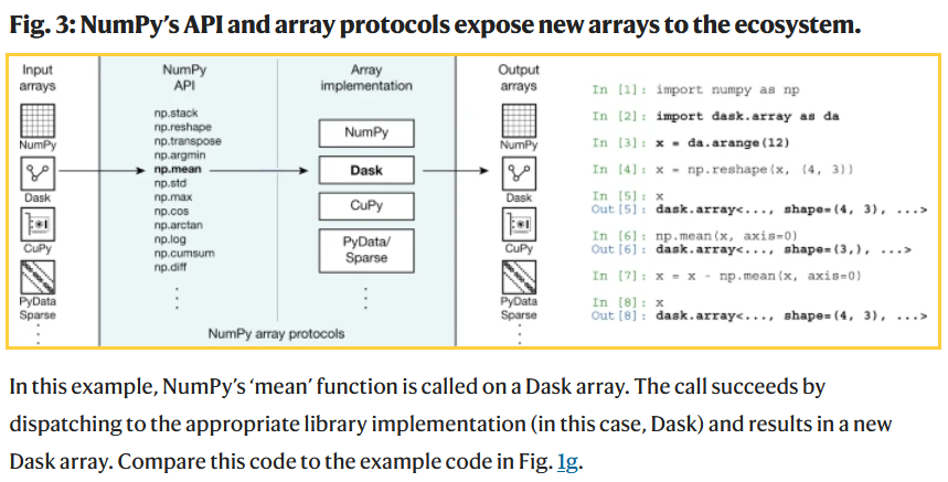
Harris, Charles R., et al. "Array programming with NumPy." nature 585.7825 (2020): 357-362.
Dask = python parallel computing library for cluster computing (e.g., at Google etc).
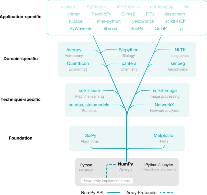
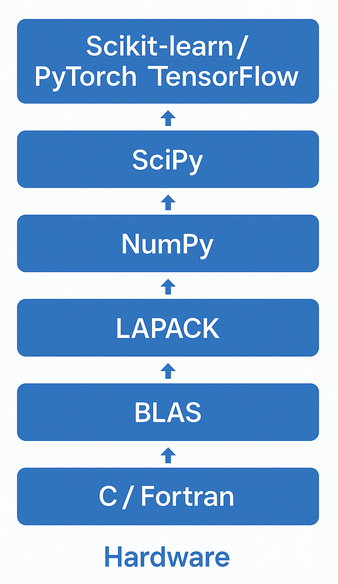
Many popular packages (include popular AI frameworks) are built upon Numpy or "swappable" replacements.
Harris, Charles R., et al. "Array programming with NumPy." nature 585.7825 (2020): 357-362.
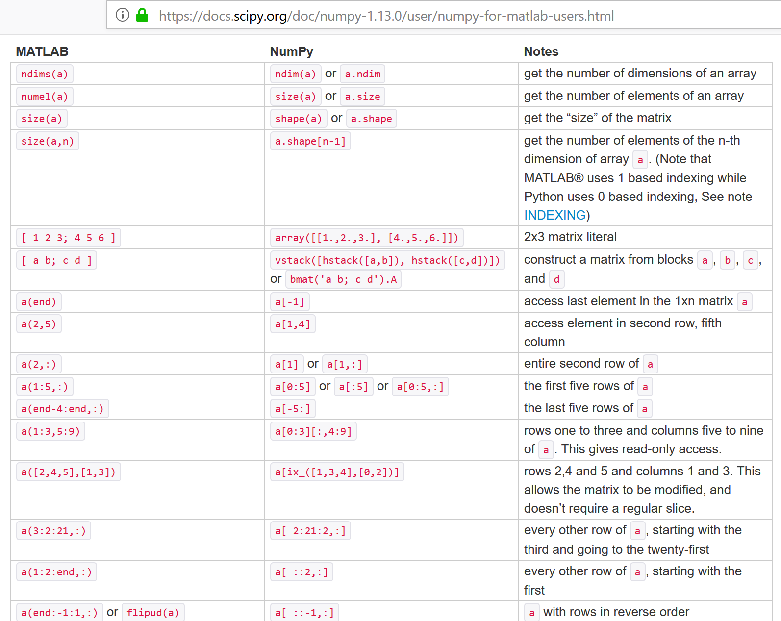
Note that numpy didn't invent everything. It primarily imitated matlab syntax. For the fast algorithm implementations it utilized the same (national lab created) open-source linear algebra libraries that were the basis for matlab.
View as wrappers for python lists, similar to our vector class.
import numpy as np

lst = [2,0,1,8]
x = np.array(lst)
x
array([2, 0, 1, 8])
type(x)
numpy.ndarray
#help(np.array)
It is very common to import numpy with alias 'np', then call functions using 'np.' prefix. It typically gives access to everything in the module and its submodules (np.random, np.linalg), but may not if they are large and not included by default.
import numpy as np
arr = np.array([1,2,3,4])
You can also import the classes individually
from numpy import array
arr = array([1,2,3,4])
lst = list([1,2,3,4])
You can also import everything, though this risks overwriting names you use. Ultimately they are just more classes like the vector class we created.
from numpy import *
np.array([2,0,1,8]) + np.array([1,1,1,1])
array([3, 1, 2, 9])
list([2,0,1,8]) + list([1,1,1,1])
[2, 0, 1, 8, 1, 1, 1, 1]
# "Array programming"

x = np.array([2,0,1,8])
y = np.array([1,1,1,1])

z = x + y
print(z)
[3 1 2 9]
v = np.array([1,2,3])
w = np.array([3,4,5])


print(5*v+3*w)
print(5*(v + 3*w) + w + 1) # note scalar addition also
[14 22 30]
[54 75 96]
3 * np.array([2,0,1,8])
array([ 6, 0, 3, 24])
3 * list([2,0,1,8])
[2, 0, 1, 8, 2, 0, 1, 8, 2, 0, 1, 8]
This can be defined a number of ways in linear algebra (e.g. $\mathbf x^T \mathbf y$). Will return to this later.
w = np.array([1, 2])
v = np.array([3, 4])
np.dot(w,v)
11
w = np.array([0, 1])
v = np.array([1, 0])
np.dot(w,v)
0
w = np.array([1, 2])
v = np.array([-2, 1])
np.dot(w,v)
0
NumPy arrays are zero-based like Python lists
x = np.array([2,0,1,8])

print(x)
print(x[0],x[3])
[2 0 1 8]
2 8
Also slicing is similar
print(x[0:3])
[2 0 1]
Numpy arrays are classes with their own type
The data can be of various types.
type(x), type(x[0])
(numpy.ndarray, numpy.int32)
x = np.array([2,0,1,8], dtype=np.int64)
type(x), type(x[0])
(numpy.ndarray, numpy.int64)
Various combinations of short vs long (or single versus double) int versus float, signed versus unsigned (for ints).
Details depends on platform (Linux vs Windows vs Mac vs Andriod..) and has evolved over time.
| Common names | bits | Python name | Numpy name(s) |
|---|---|---|---|
| boolean (bool) | 8 | numpy.bool | |
| character (char) | 8 | numpy.char | |
| integers (int) | 32 | int | numpy.intc, numpy.int32 |
| unsigned integers (uint) | 32 | numpy.uint32 | |
| floating-pointing numbers (float, single) | 32,64 | float | numpy.float32, numpy.float64 |
| double precision floating point numbers (double) | 64 | numpy.double | |
| short integers (short) | 16 | numpy.short | |
| long integers (long) | 32,64 | numpy.long | |
| double long integers (longlong) | 64,128? | numpy.longlong | |
| unsigned long integers (ulong) | 32,64 | numpy.ulong |
https://en.cppreference.com/w/cpp/language/types </br> https://numpy.org/devdocs/user/basics.types.html
import numpy

-1.0*numpy.float32(0.0)
-0.0
import numpy

-1./numpy.float32(0.)
C:\Users\micro\AppData\Local\Temp\ipykernel_29412\4148764609.py:3: RuntimeWarning: divide by zero encountered in true_divide
  -1./numpy.float32(0.)
-inf
0.0/numpy.float32(0.0)
C:\Users\micro\AppData\Local\Temp\ipykernel_29412\3555820988.py:1: RuntimeWarning: invalid value encountered in true_divide
  0.0/numpy.float32(0.0)
nan
0*numpy.nan
nan
numpy.inf*numpy.nan
nan
numpy.inf == 1/numpy.float32(0.0)
C:\Users\micro\AppData\Local\Temp\ipykernel_29412\2350908150.py:1: RuntimeWarning: divide by zero encountered in true_divide
  numpy.inf == 1/numpy.float32(0.0)
True
numpy.nan == numpy.nan # !!
False
numpy.isnan(numpy.float32(0)/numpy.float32(0))
C:\Users\micro\AppData\Local\Temp\ipykernel_29412\4269917502.py:1: RuntimeWarning: invalid value encountered in float_scalars
  numpy.isnan(numpy.float32(0)/numpy.float32(0))
True
numpy.isinf(1.0/numpy.float32(0))
C:\Users\micro\AppData\Local\Temp\ipykernel_29412\468334143.py:1: RuntimeWarning: divide by zero encountered in true_divide
  numpy.isinf(1.0/numpy.float32(0))
True
Converting loops into linear algebra functions where loop is performed at lower level
E.g. instead of looping over lists, use preprogrammed fast operations on arrays
x = range(0,1000)
alpha = 5

%timeit ax = list([alpha*x_k for x_k in x])
99.1 µs ± 10.5 µs per loop (mean ± std. dev. of 7 runs, 10000 loops each)
import numpy as np
x = np.arange(0,1000) # <-- conceptually same as np.array(range(0,1000))
alpha = 5

%timeit ax = alpha*x
1.75 µs ± 433 ns per loop (mean ± std. dev. of 7 runs, 100000 loops each)
https://numpy.org/doc/stable/reference/ufuncs.html
Many common operations are implemented efficiently in numpy on elementwise basis
type(np.cos)
numpy.ufunc
v = np.array([1,2,3,4])
np.cos(np.array(v))
array([ 0.54030231, -0.41614684, -0.9899925 , -0.65364362])
np.log(np.array(v))
array([0. , 0.69314718, 1.09861229, 1.38629436])
np.exp([1,2,3,4]) # note can pass in lists
array([ 2.71828183, 7.3890561 , 20.08553692, 54.59815003])
np.add((1,2,3,4),(5,6,7,8)) # or tuples
array([ 6, 8, 10, 12])
Many are also supported via dunders for array programming
v = [1,2,3,4,5]

np.power(v,2), np.array(v)**2, np.array(v).__pow__(2)
(array([ 1,  4,  9, 16, 25], dtype=int32),
 array([ 1,  4,  9, 16, 25], dtype=int32),
 array([ 1,  4,  9, 16, 25], dtype=int32))
v = range(0,1000)

%timeit v2 = list([x**2 for x in v])
266 µs ± 7.21 µs per loop (mean ± std. dev. of 7 runs, 1000 loops each)
import numpy as np
v = np.arange(0,1000)

%timeit v2 = v**2
1.33 µs ± 18.4 ns per loop (mean ± std. dev. of 7 runs, 1000000 loops each)
https://numpy.org/doc/stable/reference/generated/numpy.vectorize.html
f_vectorized = np.vectorize(f)
import numpy as np
import math

def myfun(x):
    if x>0:
        return math.sqrt(x)
    else:
        return 0

myvfun = np.vectorize(myfun)

myvfun([1,2,3,4])
array([1. , 1.41421356, 1.73205081, 2. ])
A matrix $\mathbf A$ is a rectangular array of numbers, of size $m \times n$ as follows:
$\mathbf A = \begin{bmatrix} A_{1,1} & A_{1,2} & A_{1,3} & \dots & A_{1,n} \\ A_{2,1} & A_{2,2} & A_{2,3} & \dots & A_{2,n} \\ \vdots & \vdots & \vdots & \ddots & \vdots \\ A_{m,1} & A_{m,2} & A_{m,3} & \dots & A_{m,n} \end{bmatrix}$
Where the numbers $A_{ij}$ are called the elements of the matrix. We describe matrices as wide if $n > m$ and tall if $n < m$. They are square iff $n = m$.
NOTE: naming convention for scalars vs. vectors vs. matrices.
Modern computer memory is one-dimensional, so must define meaning of rows vs columns
List of lists (but is it a list of rows or of columns?)
A = [[1,2,3],[4,5,6],[7,8,9]]
How do you select the $(i,j)$th element?
What if we simply stored the matrix $A$ as a 1d Array? Now how do you select the $(i,j)$th element?
Can convert that list of lists into a numpy matrix
A = [[1,2,3],[4,5,6],[7,8,9]]

import numpy as np
np.array(A)
array([[1, 2, 3],
       [4, 5, 6],
       [7, 8, 9]])
import numpy as np

np.matrix([[1,2,3],[4,5,6],[7,8,9]])
matrix([[1, 2, 3],
        [4, 5, 6],
        [7, 8, 9]])
https://numpy.org/doc/stable/reference/generated/numpy.matrix.html
"Note: It is no longer recommended to use this class, even for linear algebra. Instead use regular arrays. The class may be removed in the future."
https://stackoverflow.com/questions/53254738/deprecation-status-of-the-numpy-matrix-class
import numpy as np
np.array([[1,2,3],[4,5,6],[7,8,9]])
array([[1, 2, 3],
       [4, 5, 6],
       [7, 8, 9]])
np.array([[[1,2,3],[4,5,6],[7,8,9]],[[0,2,0],[4,0,6],[0,8,9]]])
array([[[1, 2, 3],
        [4, 5, 6],
        [7, 8, 9]],

       [[0, 2, 0],
        [4, 0, 6],
        [0, 8, 9]]])
the length of the "raw data"
np.array([2,0,1,8]).size
4
np.array([[[2,0,1,8]]]).size
4
np.array([[[1,2,3],[4,5,6],[7,8,9]],[[0,2,0],[4,0,6],[0,8,9]]]).size
18
the number of dims. Think of as number of nested lists
np.array([2,0,1,8]).ndim
1
np.array([[[1,2,3],[4,5,6],[7,8,9]],[[0,2,0],[4,0,6],[0,8,9]]]).ndim
3
np.array([[2,0,1,8]]).ndim
2
np.array([[[2,0,1,8]]]).ndim
3
If view $A$ as a $m \times n$ matrix, A.shape returns a tuple $(m,n)$
A = np.array([[1,2],[4,5],[7,8]])

print(A)
print('')
print(A.shape)
[[1 2]
 [4 5]
 [7 8]]

(3, 2)
Note if view as list of lists, shape elements are outermost list size first
T = np.array([[[1,2],[3,4],[5,6],[1,2],[3,4],[5,6]],[[1,2],[3,4],[5,6],[1,2],[3,4],[5,6]]])
print(T)
print('')
print(T.shape)
[[[1 2]
  [3 4]
  [5 6]
  [1 2]
  [3 4]
  [5 6]]

 [[1 2]
  [3 4]
  [5 6]
  [1 2]
  [3 4]
  [5 6]]]

(2, 6, 2)
np.array([1,2,3,4]).shape
(4,)
tuple([4])
(4,)
np.array([[1,2,3,4]]).shape
(1, 4)
np.array([[1],[2],[3],[4]]).shape
(4, 1)
print(np.array([[1,2,3,4]]))
print(np.array([[1],[2],[3],[4]]))
[[1 2 3 4]]
[[1]
 [2]
 [3]
 [4]]
Similar to lists. Supports index tuples also
A = np.array([[1,2,3],[4,5,6],[7,8,9]])
print(A)
[[1 2 3]
 [4 5 6]
 [7 8 9]]
print(A[1][2]) # list-of-list style (zero-based of course)
6
print(A[1,2]) # tuple style (also matlab)
6
print(A[(1,2)]) # explicit tuple
6
print(A)
print('')
print(A[:,0]) # slice all rows, 3th column ~ A[0:3,0]
[[1 2 3]
 [4 5 6]
 [7 8 9]]

[1 4 7]
print(A[1,:])
[4 5 6]
print(A)
print('')

print(A[1][:]) # ok
[[1 2 3]
 [4 5 6]
 [7 8 9]]

[4 5 6]
print(A[:][0]) # wrong!
[1 2 3]
what did this do? hint: view as (A[:])[0]
print(A)
print('')

print(A[1:,0:2])
[[1 2 3]
 [4 5 6]
 [7 8 9]]

[[4 5]
 [7 8]]
print(A[:2,:2])
[[1 2]
 [4 5]]
print(A)
print('')
print(A[:,0:1])
[[1 2 3]
 [4 5 6]
 [7 8 9]]

[[1]
 [4]
 [7]]
print(A[:,0])
[1 4 7]
mask = np.array([[True, True, False],[True,True,False],[False,False,False]])
print(mask)
[[ True  True False]
 [ True  True False]
 [False False False]]
print(A)
print('')
A[mask]
[[1 2 3]
 [4 5 6]
 [7 8 9]]
array([1, 2, 4, 5])
Notice it comes out flat
handy when combined with logic
v = np.arange(10)
print(v)
print(v>=5)
print(v[v>=5])
[0 1 2 3 4 5 6 7 8 9]
[False False False False False  True  True  True  True  True]
[5 6 7 8 9]
A.flatten() - returns flattened copy
A.ravel() - returns reference of original, but as if flat
A = np.array([[1,2,3],[4,5,6]])

print(A)

A.flatten(), A.shape, A.flatten().shape # note returned, not in-place
[[1 2 3]
 [4 5 6]]
(array([1, 2, 3, 4, 5, 6]), (2, 3), (6,))
A.ravel(), A.shape, A.ravel().shape # note returned, not in-place
(array([1, 2, 3, 4, 5, 6]), (2, 3), (6,))
A.flatten()[4], A.ravel()[4]
(5, 5)
aflat = A.flatten()

aflat[0] = -1
print(A)
print(aflat)
[[1 2 3]
 [4 5 6]]
[-1  2  3  4  5  6]
arav = A.ravel()

arav[0] = -1
print(A)
print(arav)
[[-1  2  3]
 [ 4  5  6]]
[-1  2  3  4  5  6]
This kind of reference to same memory but treating as if different shape is called a "view".
A.reshape(N,M,...)
A = np.array([[1,2,3],[4,5,6]])
print(A)
[[1 2 3]
 [4 5 6]]
x = np.array([1,2,3,4])
x = x.reshape(4,1) # note returned, not in-place
print(x)
[[1]
 [2]
 [3]
 [4]]
x = np.array([1,2,3,4])
x = x.reshape(4,) # note returned, not in-place
print(x)
[1 2 3 4]
print(x.reshape(2,2))
[[1 2]
 [3 4]]
print(x.reshape(1,1,2,2))
[[[[1 2]
   [3 4]]]]
Three ways: A.T, A.transpose(), np.transpose(A)
x = np.array([[1,2,3]])
print(x)
print(x.T)
print(x.transpose())
print(np.transpose(x))
[[1 2 3]]
[[1]
 [2]
 [3]]
[[1]
 [2]
 [3]]
[[1]
 [2]
 [3]]
x = np.array([[1,2,3]])
print(x)
print(x.T)
print (x.shape, x.T.shape)
[[1 2 3]]
[[1]
 [2]
 [3]]
(1, 3) (3, 1)
x = np.array([1,2,3,4])
print(x)
print(x.T)
print(x.shape, x.T.shape)
[1 2 3 4]
[1 2 3 4]
(4,) (4,)
ufuncs again
sizes must agree.
Scalar Multiplication: $\textit{B} = \alpha\ \textit{A}$ or $\textit{B} = \textit{A} \alpha$ with components $b_{ij} = \alpha a_{ij}$.
Matrix Addition: $\textit{C} = \textit{A} + \textit{B}$ with components $c_{ij} = a_{ij}+b_{ij}$.
Hadamard product (aka elementwise product): $\textit{C} = \textit{A} \odot \textit{B}$ with components $c_{ij} = a_{ij}b_{ij}$.
Can easily implement these manually on a list of lists by looping over elements
use numpy array programming to demonstrate an example for each of these
Recall scalar-vector addition, it seems natural to do the following
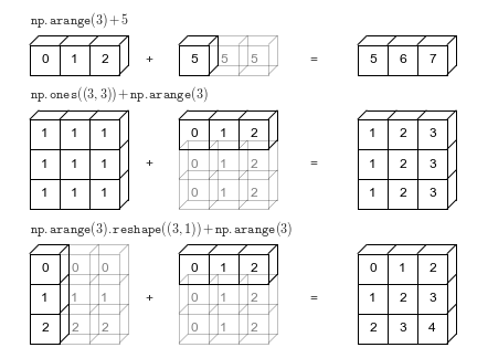
$$ \alpha + \textbf{x} \;\;\; \rightarrow \;\;\; \alpha + \begin{bmatrix} x_1 \\x_2 \\ \vdots \\ x_k \end{bmatrix} \;\;\; \leftrightarrow \;\;\; \begin{bmatrix} \alpha + x_1 \\\alpha + x_2 \\ \vdots \\ \alpha + x_k \end{bmatrix} $$view as combination of broadcasting of scalar to vector, following by vector-vector addition (i.e., elementwise addition)
$$ \alpha + \begin{bmatrix} x_1 \\x_2 \\ \vdots \\ x_k \end{bmatrix} \;\;\; \rightarrow \;\;\; \begin{bmatrix} \alpha \\\alpha \\ \vdots \\ \alpha \end{bmatrix} + \begin{bmatrix} x_1 \\x_2 \\ \vdots \\ x_k \end{bmatrix} = \begin{bmatrix} \alpha + x_1 \\\alpha + x_2 \\ \vdots \\ \alpha + x_k \end{bmatrix} $$Add (or Multiply) matrices or vectrors in an element-wise manner by repeating "singular" dimensions.
Matlab and Numpy automatically do this now.
Also (and previously) in matlab, e.g.: "brcm(@plus, A, x). numpy.broadcast
w = np.array([[2,-6],[-1, 4]])
v = np.array([1,0])

print(w)
print('')
print(w+v)
[[ 2 -6]
 [-1  4]]

[[ 3 -6]
 [ 0  4]]
print(w*v)
[[ 2  0]
 [-1  0]]
print(np.multiply(w,v)) # ufunc version. supports broadcasting
[[ 2  0]
 [-1  0]]
If $A$ is an $m \times n$ matrix and $\mathbf{v}$ is a vector of size $n$:
$$\mathbf{b} = A \mathbf{v}$$$$b_i = (A \mathbf{v})_i = \sum_{j=1}^{n} a_{ij} v_j $$Linear combination of columns
Dot product of vector with rows of matrix
$\begin{bmatrix} 2 & -6 \\ -1 & 4\\ \end{bmatrix} \begin{bmatrix} 2 \\ -1 \\ \end{bmatrix} = ?$
Test both ways out.
You can easily implement both approaches with your vector class
Can view a matrix as list of rows or list of columns
Hence can view this system two different ways.
where $\mathbf a^{(i)}$ are rows of $\mathbf A$
where $\mathbf a_1$ are columns of $\mathbf A$.
A special case of matrix-matrix multiplication (coming up)
A = np.array([[1,2,3],[4,5,6],[7,8,9]])

v = np.array([1,0,0])

A@v # array programming approach
array([1, 4, 7])
np.matmul(A,v)
array([1, 4, 7])
np.dot(A,v)
array([1, 4, 7])
what is the rule for shape matching in these products?
A = np.array([[1,2,3],[4,5,6],[7,8,9]])
x = np.array([1,0,0])
print(A,'\n')
print(x,'\n')
print(A@x,'\n') # right multiply (implies column vector)
print(x@A) # left multiply (implies row vector)
[[1 2 3]
 [4 5 6]
 [7 8 9]]

[1 0 0]

[1 4 7]

[1 2 3]
Multiplication of an $m \times n$ matrix $\textit{A}$ and a $n \times k$ matrix $\textit{B}$ is a $m \times k$ matrix $\textit{C}$, written $\textit{C} = \textit{A}\textit{B}$, whose elements $C_{ij}$ are
$$ C_{i,j} = \sum_{l=1}^n A_{i,l}B_{l,j} $$Note that $\textit{B}\textit{A} \neq \textit{A}\textit{B}$ in general.
$\textit{C} = \textit{A}\textit{B} = \begin{bmatrix} 1 & 2 \\ 0 & 1 \\ \end{bmatrix} \begin{bmatrix} 2 & 0 \\ 1 & 4 \\ \end{bmatrix} = \begin{bmatrix} 4 & 8 \\ 1 & 4 \\ \end{bmatrix}$
$\begin{bmatrix} 1 & 2 \\ 0 & -3 \\ 3 & 1 \\ \end{bmatrix} \begin{bmatrix} 2 & 6 & -3 \\ 1 & 4 & 0 \\ \end{bmatrix} = ?$
A = np.array([[1,2],[3, 4]])
B = np.array([[1,0],[2, 1]])
print(A@B)
[[ 5  2]
 [11  4]]
print(np.matmul(A,B))
[[ 5  2]
 [11  4]]
print(np.dot(A,B))
[[ 5  2]
 [11  4]]
A = np.array([[ 2, -6],
              [-1,  4]])

x = np.array([[+1],
              [-1]])
A@x
array([[ 8],
       [-5]])
x@A
---------------------------------------------------------------------------
ValueError                                Traceback (most recent call last)
~\AppData\Local\Temp\ipykernel_7112\299605771.py in <module>
----> 1 x@A

ValueError: matmul: Input operand 1 has a mismatch in its core dimension 0, with gufunc signature (n?,k),(k,m?)->(n?,m?) (size 2 is different from 1)
vrow = np.array([[1,2,3,4]])
print(vrow)
vcol = np.array([[1],[2],[3],[4]])
print(vcol)
[[1 2 3 4]]
[[1]
 [2]
 [3]
 [4]]
vrow@vcol
array([[30]])
vcol@vrow
array([[ 1,  2,  3,  4],
       [ 2,  4,  6,  8],
       [ 3,  6,  9, 12],
       [ 4,  8, 12, 16]])
np.array([1,2,3,4])@np.array([1,2,3,4]) # 1D arrays - treated as inner product
30
np.zeros((3,4))
array([[0., 0., 0., 0.],
       [0., 0., 0., 0.],
       [0., 0., 0., 0.]])
np.ones((3,4))
array([[1., 1., 1., 1.],
       [1., 1., 1., 1.],
       [1., 1., 1., 1.]])
D = np.diag([1,2,3])
print(D)
[[1 0 0]
 [0 2 0]
 [0 0 3]]
np.diag(D)
array([1, 2, 3])
$I_3 = \begin{bmatrix} 1 & 0 & 0\\ 0 & 1 & 0 \\ 0 & 0 & 1\\ \end{bmatrix}$
Here we can write $\textit{I}\textit{B} = \textit{B}\textit{I} = \textit{B}$ or $\textit{I}\textit{I} = \textit{I}$
Again, it is important to reiterate that matrices are not in general commutative with respect to multiplication. That is to say that the left and right products of matrices are, in general different.
$AB \neq BA$
import numpy as np
np.eye(3)
array([[1., 0., 0.],
       [0., 1., 0.],
       [0., 0., 1.]])
# rand = uniform random numbers in [0,1]

np.random.rand(3,4) # note two inputs, not tuple
array([[0.99147344, 0.01075122, 0.81974321, 0.10942128],
       [0.94041317, 0.50408574, 0.71896232, 0.12113072],
       [0.77483078, 0.32627551, 0.44489225, 0.13208849]])
# randn ~ N(0,1)

np.random.randn(3,4)
array([[ 1.09642959,  1.40715723, -0.30932909,  0.66846735],
       [ 0.22536484, -0.08283707, -0.60713286, -0.16836462],
       [-1.20191307,  1.53390883, -0.48587343, -0.84379159]])
What is the product of $\begin{bmatrix} 2 & -6 \\ -1 & 4\\ \end{bmatrix}$ and $\begin{bmatrix} -1 & 1 \\ \end{bmatrix}$ in python?
If question seems vague, list all possible ways to address this question.
Implement the "linear algebra with Python" Exercises from the bootcamp using numpy:
https://www.keithdillon.com/classes/UMMC/Bootcamp/__python_exercises_01.html
Many popular packages (include popular AI frameworks) are built upon Numpy or "swappable" replacements.
Harris, Charles R., et al. "Array programming with NumPy." nature 585.7825 (2020): 357-362.
Harris, Charles R., et al. "Array programming with NumPy." nature 585.7825 (2020): 357-362.
Dask = python parallel computing library for cluster computing (e.g., at Google etc).
https://docs.scipy.org/doc/numpy/reference/routines.linalg.html