Many popular packages (include popular AI frameworks) are built upon Numpy or "swappable" replacements.
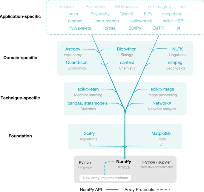
Harris, Charles R., et al. "Array programming with NumPy." nature 585.7825 (2020): 357-362.
The most common Python visualization tool
A module within matplotlib which provides a relatively-simple interface, modelled after matlab.
Can be used in direct "state-based" calls, closest to matlab-style:
import numpy as np
import matplotlib.pyplot as plt

x = np.arange(0, 15, 0.1)
y = np.sin(x)
plt.figure()
plt.plot(x, y)
plt.show()

For much more control and features, you must directly access the pytorch classes via object-oriented API
Usually necessary to get a plot to look exactly the way you want it.
import matplotlib.pyplot as plt

fig, ax = plt.subplots()

fruits = ['apple', 'blueberry', 'cherry', 'orange']
counts = [40, 100, 30, 55]
bar_labels = ['red', 'blue', '_red', 'orange']
bar_colors = ['tab:red', 'tab:blue', 'tab:red', 'tab:orange']

ax.bar(fruits, counts, label=bar_labels, color=bar_colors)
ax.set_ylabel('fruit supply')
ax.set_title('Fruit supply by kind and color')
ax.legend(title='Fruit color')
plt.show()

Jupyter has built-in magic function: the "matoplotlib inline" mode, which will draw the plots directly inside the notebook. Should be on by default.
%matplotlib inline
Without this mode, or in ipython, use .show() function to generate visualization
plt.show()
Accepts various types of inputs (list, array, ...)
plt.plot([0,1,-2,3,-4,5]);

plot x versus y
x = np.linspace(0, 10, 100)
y = np.sin(x)
plt.plot(x, y);

Colors automatically changed for multiple traces
x = np.linspace(0, 10, 100)
plt.plot(x, np.sin(x));
plt.plot(x, np.sin(x)+0.5);
plt.plot(x, np.sin(x)+1);

Or select trace style
x = np.linspace(0, 10, 100)
plt.plot(x, np.sin(x) ,    'ko');
plt.plot(x, np.sin(x)+0.5, 'rs');
plt.plot(x, np.sin(x)+1,   'g.');

x = np.random.normal(size=500)
y = np.random.normal(size=500)
plt.scatter(x, y);

Can be $M\times N$ matrices or $M\times N \times 3$ arrays representing color
note that origin is at the top-left by default
im = np.array([[1, 2, 3],[4,5,6],[6,7,8]])
import matplotlib.pyplot as plt

plt.imshow(im);
plt.colorbar();
plt.xlabel('x')
plt.ylabel('y');

note that origin here is at the bottom-left by default
plt.contour(im);

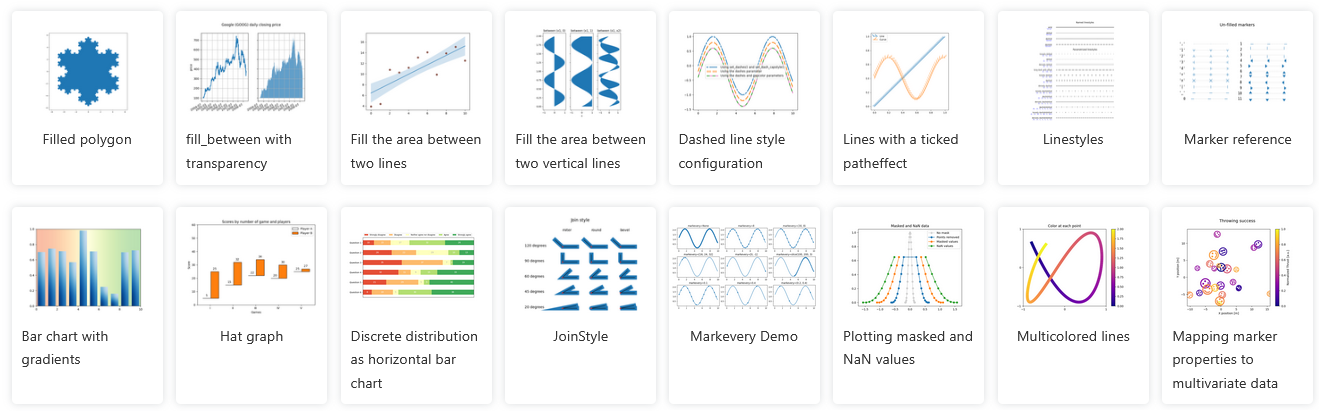
There are many more plot types available.
See matplotlib gallery] at http://matplotlib.org/gallery.html
To run, copy the Source Code link near bottom of page, and put it in a notebook using the %load magic.
%load <link goes here>
Then run cell
%load http://matplotlib.org/mpl_examples/pylab_examples/ellipse_collection.py
call plt.savefig(filename) after forming plot.
https://matplotlib.org/stable/api/_as_gen/matplotlib.pyplot.savefig.html
plt.plot([0,1,-2,3,-4,5]);
plt.savefig("test_savefig_example.pdf") # png, jpg, ...
To achieve nice-looking figures often requires a lot of code as you must specify every detail of the figure carefully.
You may find yourself having to go back and research how to achieve each detail whenever it comes time to publish.
Alternatives:
Extends NumPy providing additional tools for array computing and provides specialized data structures, such as sparse matrices and k-dimensional trees.
Wraps highly-optimized implementations written in low-level languages like Fortran, C, and C++.
import scipy
printcols(dir(scipy),2)
LowLevelCallable   ndimage
__numpy_version__  odr
__version__        optimize
cluster            show_config
fft                signal
fftpack            sparse
integrate          spatial
interpolate        special
io                 stats
linalg             test
misc
import numpy.linalg
#[fun for fun in dir(numpy.linalg) if not fun.startswith('_')]
import scipy.linalg
#[fun for fun in dir(scipy.linalg) if not fun.startswith('_')]
from scipy.stats import norm

print(norm.pdf(0))
print(norm.cdf(1))
print(norm.rvs(size=10)) # random samples
0.3989422804014327
0.8413447460685429
[ 0.85099468 -0.82656877 -0.09945668 -0.07761511 -0.59359535 -2.48334685
 -1.16963941  0.55575344  0.62577528  1.06376605]
#printcols([fun for fun in dir(scipy.stats) if not fun.startswith('_')],4)
from scipy.optimize import minimize
import numpy as np

def f(x):
    return (x - 3)**2

res = minimize(f, x0=0)
res
      fun: 2.5388963550532293e-16
 hess_inv: array([[0.5]])
      jac: array([-1.69666681e-08])
  message: 'Optimization terminated successfully.'
     nfev: 6
      nit: 2
     njev: 3
   status: 0
  success: True
        x: array([2.99999998])
printcols([fun for fun in dir(scipy.optimize) if not fun.startswith('_')],4)
BFGS                      brute                     fsolve                    nnls
Bounds                    check_grad                golden                    nonlin
HessianUpdateStrategy     cobyla                    lbfgsb                    optimize
LbfgsInvHessProduct       curve_fit                 least_squares             quadratic_assignment
LinearConstraint          diagbroyden               leastsq                   ridder
NonlinearConstraint       differential_evolution    line_search               root
OptimizeResult            direct                    linear_sum_assignment     root_scalar
OptimizeWarning           dual_annealing            linearmixing              rosen
RootResults               excitingmixing            linesearch                rosen_der
SR1                       fixed_point               linprog                   rosen_hess
anderson                  fmin                      linprog_verbose_callback  rosen_hess_prod
approx_fprime             fmin_bfgs                 lsq_linear                shgo
basinhopping              fmin_cg                   milp                      show_options
bisect                    fmin_cobyla               minimize                  slsqp
bracket                   fmin_l_bfgs_b             minimize_scalar           test
brent                     fmin_ncg                  minpack                   tnc
brenth                    fmin_powell               minpack2                  toms748
brentq                    fmin_slsqp                moduleTNC                 zeros
broyden1                  fmin_tnc                  newton
broyden2                  fminbound                 newton_krylov
Machine Learning functions. Previously dominant Machine Learning toolbox.
Was getting discarded as field switched from single CPU to GPU and distributed, but making comeback with upgrades for scaling sizes and parallelism
Given training data $(\mathbf x_{(i)},y_i)$ for $i=1,...,m$ --> lists of samples $\mathbf X$ and labels $\mathbf y$
Choose a model $f(\cdot)$ where we want to make $f(\mathbf x_{(i)})\approx y_i$ (for all $i$) --> choose sklearn estimator to use
Define a loss function $L(f(\mathbf x), y)$ to minimize by changing $f(\cdot)$ ...by adjusting the weights --> default choices for estimators, sometimes multiple options
In traditional machine learning the models were support vector machines, decision trees, various kinds of regression models (linear, polynomial, logistic).
In modern AI they are deep learning "architectures".
Unlike traditional statistics, Machine Learning is about making a tool to predict things, as opposed to doing science or data analysis. Once we have a "fit" a model, we want to use it on new data to make decisions
$$f(\mathbf x_{new})\approx ?$$Most methods have no way to compute uncertainty quantification, p-values or confidence, etc.
Scikit-learn is a uniform API over many statistical and machine learning models.
model = ModelClass(...)   # constructor. specify hyperparameters
model.fit(X, y)           # estimate model parameters from data
y_pred = model.predict(X) # generate predictions from new data
Most models/transforms/objects in sklearn are Estimator objects
class Estimator(object):

    def fit(self, X, y=None):
        """Fit model to data X (and y)"""
        self.some_attribute = self.some_fitting_method(X, y)
        return self

    def predict(self, X_test):
        """Make prediction based on passed features"""
        pred = self.make_prediction(X_test)
        return pred

model = Estimator()
The model: $$ y = \beta_0 + \beta_1 x$$
Given data $(\mathbf x_{(i)},y_i)$, we want to fit the model, which means choose $\beta_0$ and $\beta_1$.
import numpy as np
from sklearn.linear_model import LinearRegression

X = np.array([[1], [2], [3], [4], [5]])   # features (list of lists convention)
y = np.array([2, 4, 5, 4, 5])             # response
from matplotlib.pyplot import *
figure(figsize=(5,2))
plot(X,y, '.-');

#help(LinearRegression)
Scikit learn will internally compute the least squares solution
model = LinearRegression() # construct estimator class
model.fit(X, y); # fit parameters using data
print(model.coef_)      # slope
print(model.intercept_) # intercept
[0.6]
2.1999999999999993
model.score(X,y) # R^2 implemented for this model
0.6000000000000001
Here we're using the original training data to view how well it was fit
y_pred = model.predict(X)
y_pred
array([2.8, 3.4, 4. , 4.6, 5.2])
model.intercept_ + model.coef_*X
array([[2.8],
       [3.4],
       [4. ],
       [4.6],
       [5.2]])
figure(figsize=(5,2))
plot(X,y, '.-');
plot(X,y_pred, '.-');

We can apply our "trained" model to anything now
model.predict([[99]]) # note input form at list of lists of feature values
array([61.6])
model.predict([[-100]]) # note input form at list of lists of feature values
array([-57.8])
model.predict([[1e6]])
array([600002.2])
Extra info and variations for different methods are squeezed into the interface
import numpy as np
from sklearn.cluster import KMeans

# synthetic data: two clusters
X = np.array([[1, 2], [1, 3], [2, 2], [2, 3], [-8, -7], [-8, -8], [-9, -7], [-9, -8]])

figure(figsize=(5,2))
scatter(X[:,0],X[:,1]);

kmeans = KMeans(n_clusters=2, random_state=0)
kmeans.fit(X)

labels = kmeans.labels_ # cluster assignments
centers = kmeans.cluster_centers_ # cluster centers
print(centers)

figure(figsize=(5,2))
scatter(X[:,0],X[:,1]);
scatter(centers[:,0],centers[:,1]);
[[-8.5 -7.5]
 [ 1.5  2.5]]

A large focus of modern AI development is in "democratizing" the technologies.
"NVIDIA cuML is an open-source CUDA-X™ Data Science library that accelerates scikit-learn, UMAP, and HDBSCAN on GPUs—supercharging machine learning workflows with no code changes required. "
https://developer.nvidia.com/topics/ai/data-science/cuda-x-data-science-libraries/cuml
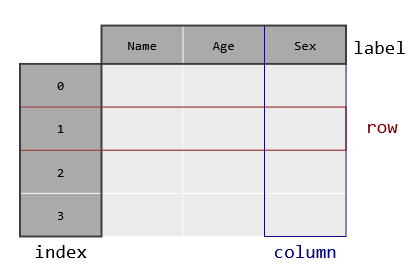
Pandas is a library for tabular data analysis built on NumPy, taking a database-style view to n-dimensional arrays (with n=2).
Pandas adds labeled axes, heterogeneous columns, and database-like data manipulation.
import numpy as np
import pandas as pd

arr = np.array([[1, 2],[3, 4]])
print(arr)
print('')
df = pd.DataFrame(arr, columns=["A", "B"], index=["r1", "r2"])
print(df)
[[1 2]
 [3 4]]

    A  B
r1  1  2
r2  3  4
df.to_numpy()
array([[1, 2],
       [3, 4]])
df.describe()
| A | B | |
|---|---|---|
| count | 2.000000 | 2.000000 |
| mean | 2.000000 | 3.000000 |
| std | 1.414214 | 1.414214 |
| min | 1.000000 | 2.000000 |
| 25% | 1.500000 | 2.500000 |
| 50% | 2.000000 | 3.000000 |
| 75% | 2.500000 | 3.500000 |
| max | 3.000000 | 4.000000 |
df = pd.DataFrame([[1, 2],[3, 4]], columns=["A", "B"], index=["r1", "r2"])
print(df)
    A  B
r1  1  2
r2  3  4
df["A"]
r1    1
r2    3
Name: A, dtype: int64
df["A"] + df["B"]
r1    3
r2    7
dtype: int64
print(df)
df.loc['r1']
    A  B
r1  1  2
r2  3  4
A    1
B    2
Name: r1, dtype: int64
df.loc['r1']+df.loc['r2']
A    4
B    6
dtype: int64
df1 = pd.DataFrame([[1, 2],[3, 4]], columns=["A", "B"], index=["r1", "r2"])
df2 = pd.DataFrame([[.1, .2],[.3, .4]], columns=["B", "C"], index=["r1", "r2"])
print(df1)
print(df2)
    A  B
r1  1  2
r2  3  4
      B    C
r1  0.1  0.2
r2  0.3  0.4
print(df1+df2)
     A    B   C
r1 NaN  2.1 NaN
r2 NaN  4.3 NaN
Each column can have its own dtype, stored as a container class of type Series()
df = pd.DataFrame({
    'age': np.array([23, 45, 31]),
    'name': ['Alice', 'Bob', 'Carol'],
    'score': [88.5, 92.0, 79.5] })
print(df)
   age   name  score
0   23  Alice   88.5
1   45    Bob   92.0
2   31  Carol   79.5
df['age']
0    23
1    45
2    31
Name: age, dtype: int32
type(df), type(df['age'])
(pandas.core.frame.DataFrame, pandas.core.series.Series)
list(df['age'])
[23, 45, 31]
df['age'].mean()
33.0
df['age'].median()
31.0
df.describe()
| age | score | |
|---|---|---|
| count | 3.000000 | 3.000000 |
| mean | 33.000000 | 86.666667 |
| std | 11.135529 | 6.448514 |
| min | 23.000000 | 79.500000 |
| 25% | 27.000000 | 84.000000 |
| 50% | 31.000000 | 88.500000 |
| 75% | 38.000000 | 90.250000 |
| max | 45.000000 | 92.000000 |
df.describe().loc['50%']
age      31.0
score    88.5
Name: 50%, dtype: float64
Many formats supported for load directly into dataframe. Also html, clipboard, parquet, feather
Corresponding .to_csv() etc methods for writing
df = pd.read_csv("data.csv")
df = pd.read_excel("data.xlsx", sheet_name="Sheet1")
df = pd.read_json("data.json")
df = pd.read_pickle("data.pkl")

import sqlite3
conn = sqlite3.connect("db.sqlite")
df = pd.read_sql("SELECT * FROM table", conn)
pandas was originally created for in-memory, single-threaded operation.
Packages like polars and NVIDIA RAPIDS use a similar interface but add support for parallel and distributed operation.
These are core methods for data science on a traditional single-CPU, in-RAM, mode of operation.
Major subsequent packages build on them to surpass their limitation.