Mathematical Methods for Data Science
Topic 5: "Classical" Linear Algebra Software
This topic:
- BLAS, LAPACK, Eigen
- Overview of major python packages
- Numpy practice
Reading: the internet
What is "Classical" Linear Algebra software?
- A term I just invented
- Originally single CPU, RAM-limited implementations of well-known algorithms (e.g. Golub & Van Loan "Matrix Computations")
- ...and higher-level packages based on these algorithms, inheriting the limitations
- Large-scale (more than 10k variable or so) only possible via sparse linear algebra algorithms
- Leading parallel tool is SIMD (single instruction multiple data) via math co-processors.
- More parallelism at top-level rather than bottom ("workers" running seperate processes on separate CPU's)
- Updates based on producing variants rather than complete replacement
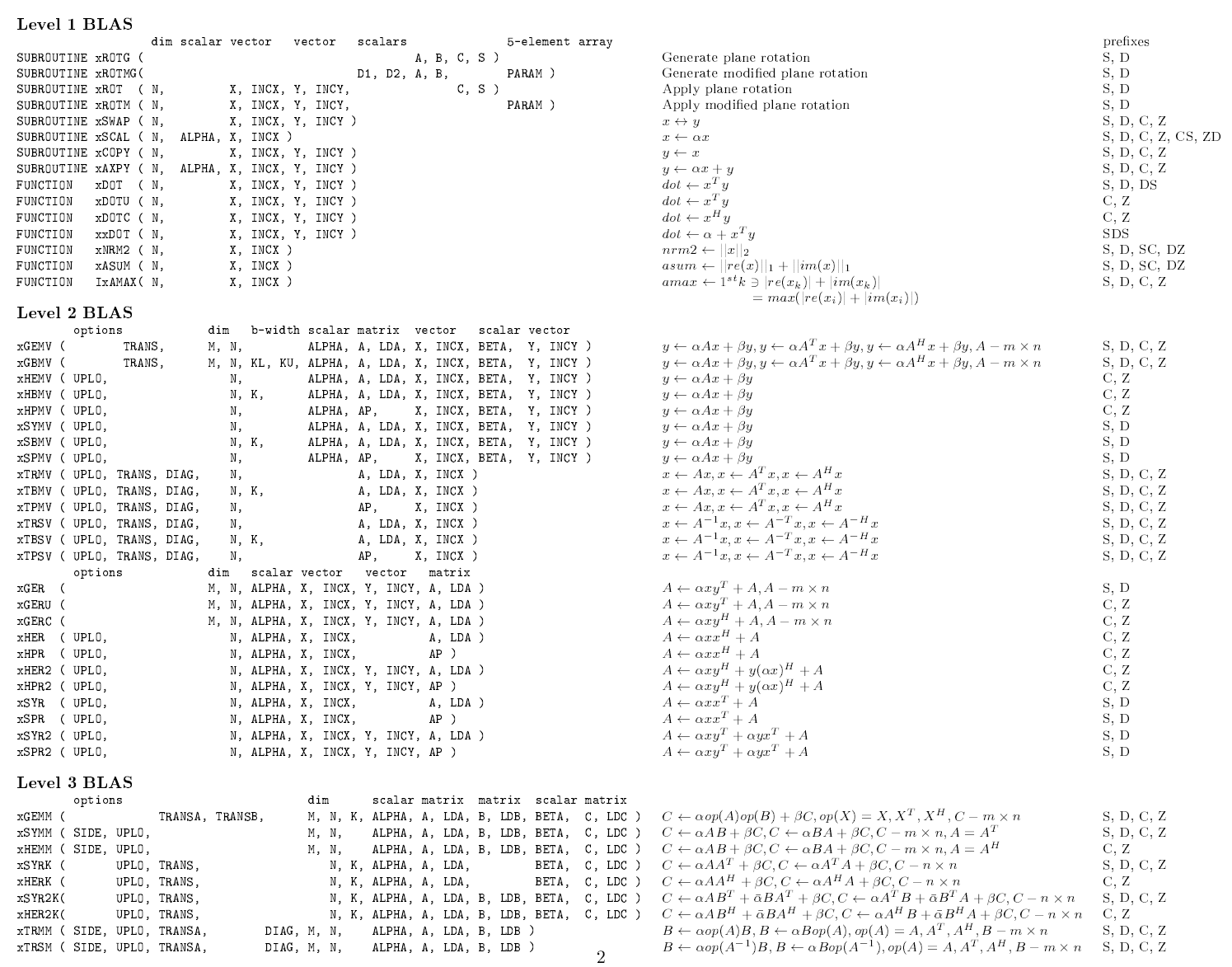
I. BLAS BLAS BLAS
BLAS = Basic Linear Algebra Subprograms
"Building block" algorithms for matrix algebra
- scaling, multiplying. "Level 1,2,3 functions"
- single and double precision, real and complex numbers
- generally don't take advantage of multiple threads or CPU's by chip maker
- Are often optimized for complex instructions however, e.g. SIMD
- Originally FORTRAN - one-based, columns first, like matlab
- various implementations, including parallelizable versions, C/C++ CUDA,
- http://www.netlib.org/blas/
More Implementations
- cuBLAS - NVIDIA https://developer.nvidia.com/cublas
- rocBLAS - AMD https://github.com/ROCm/rocBLAS?tab=readme-ov-file
- clBLAS, CLBlast - OpenCL https://github.com/CNugteren/CLBlast
- hipBLAS - a wrapper around other BLAS implementations https://github.com/ROCm/hipBLAS
- gotoBLAS, BLIS, OpenBLAS - optimized implementations for CPU https://en.wikipedia.org/wiki/GotoBLAS, https://www.openblas.net/, https://github.com/flame/blis
cuBLAS: Basic Linear Algebra on NVIDIA GPUs
https://developer.nvidia.com/cublas
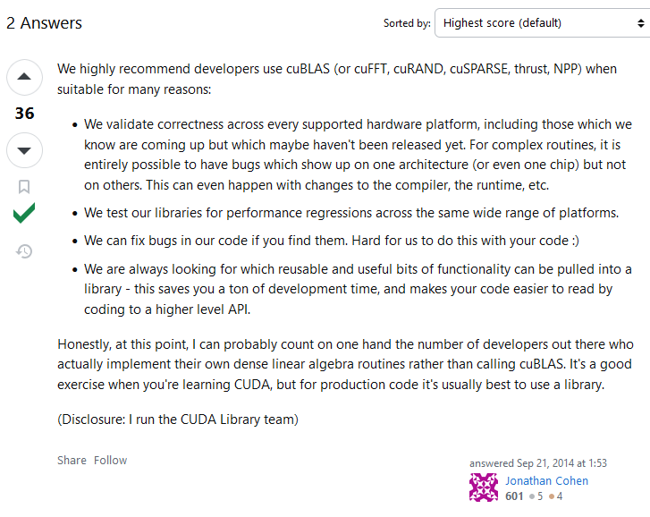
https://stackoverflow.com/questions/25836003/normal-cuda-vs-cublas
BLAS Levels 1,2,3 ~ $O(n), O(n^2), O(n^3)$
import scipy.linalg.blas as blas

printcols(dir(blas),6)
HAS_ILP64            chemm                daxpy                dtrmv                sspmv                zhbmv
__all__              chemv                dcopy                dtrsm                sspr                 zhemm
__builtins__         cher                 ddot                 dtrsv                sspr2                zhemv
__cached__           cher2                dgbmv                dzasum               sswap                zher
__doc__              cher2k               dgemm                dznrm2               ssymm                zher2
__file__             cherk                dgemv                find_best_blas_type  ssymv                zher2k
__loader__           chpmv                dger                 functools            ssyr                 zherk
__name__             chpr                 dnrm2                get_blas_funcs       ssyr2                zhpmv
__package__          chpr2                drot                 icamax               ssyr2k               zhpr
__spec__             crotg                drotg                idamax               ssyrk                zhpr2
_blas_alias          cscal                drotm                isamax               stbmv                zrotg
_cblas               cspmv                drotmg               izamax               stbsv                zscal
_fblas               cspr                 dsbmv                sasum                stpmv                zspmv
_fblas_64            csrot                dscal                saxpy                stpsv                zspr
_get_funcs           csscal               dspmv                scasum               strmm                zswap
_memoize_get_funcs   cswap                dspr                 scnrm2               strmv                zsymm
_np                  csymm                dspr2                scopy                strsm                zsyr
_type_conv           csyr                 dswap                sdot                 strsv                zsyr2k
_type_score          csyr2k               dsymm                sgbmv                zaxpy                zsyrk
caxpy                csyrk                dsymv                sgemm                zcopy                ztbmv
ccopy                ctbmv                dsyr                 sgemv                zdotc                ztbsv
cdotc                ctbsv                dsyr2                sger                 zdotu                ztpmv
cdotu                ctpmv                dsyr2k               snrm2                zdrot                ztpsv
cgbmv                ctpsv                dsyrk                srot                 zdscal               ztrmm
cgemm                ctrmm                dtbmv                srotg                zgbmv                ztrmv
cgemv                ctrmv                dtbsv                srotm                zgemm                ztrsm
cgerc                ctrsm                dtpmv                srotmg               zgemv                ztrsv
cgeru                ctrsv                dtpsv                ssbmv                zgerc
chbmv                dasum                dtrmm                sscal                zgeru
Recall: Inside the GPU
General Matrix Multiplication (GEMM) ~ $C = \alpha AB + \beta C$
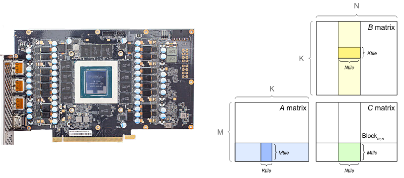
https://docs.nvidia.com/deeplearning/performance/dl-performance-matrix-multiplication/index.html
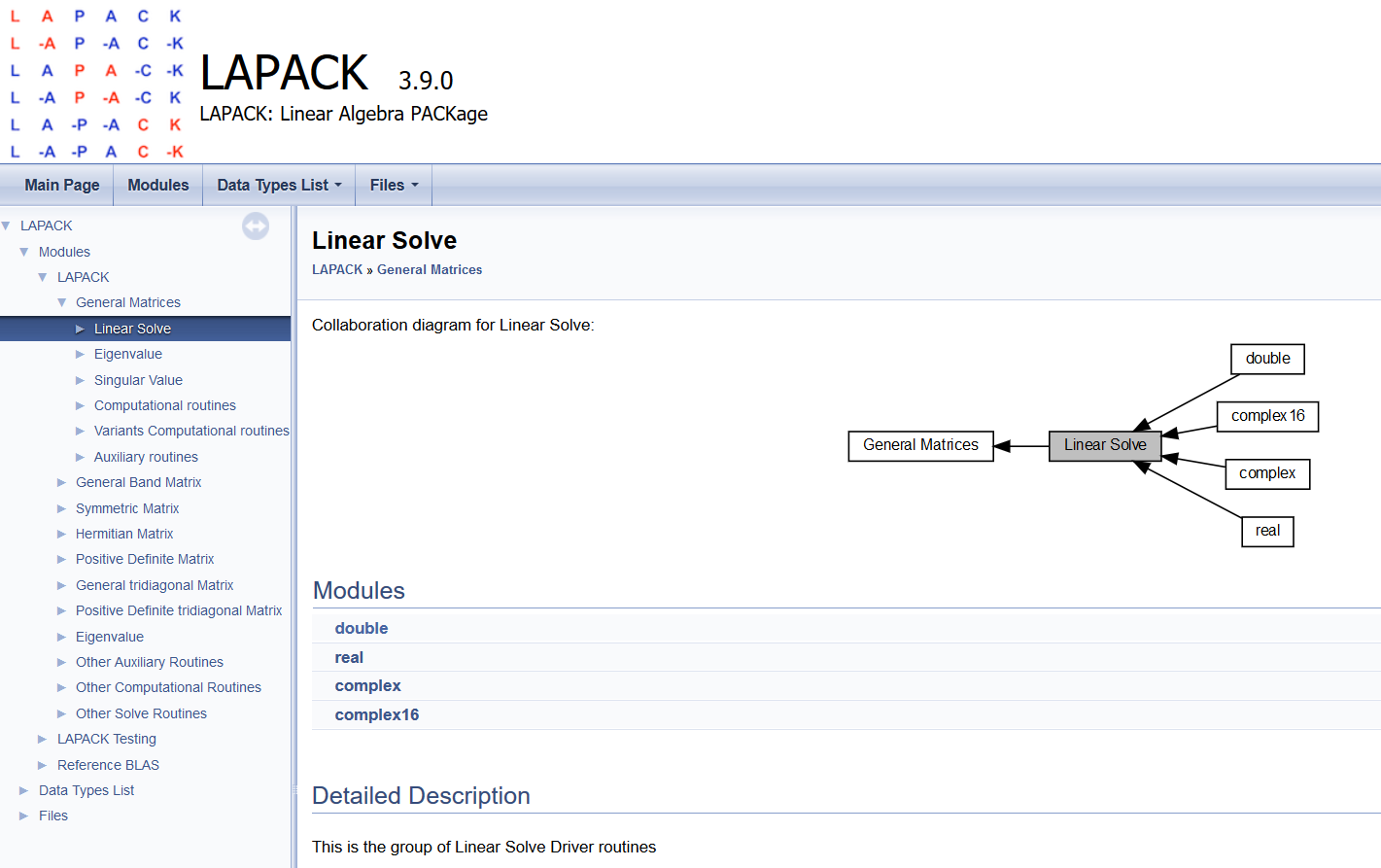
LAPACK = Linear Algebra Package
- Fortran, Uses BLAS as backend (can choose different implementations)
- http://www.netlib.org/lapack/
- https://github.com/Reference-LAPACK/lapack
- systems of simultaneous linear equations
- least-squares solutions of linear systems of equations
- eigenvalue problems
- singular value problems.
- associated matrix factorizations (LU, Cholesky, QR, SVD, Schur, generalized Schur)
- related computations such as reordering of the Schur factorizations and estimating condition numbers.
- Dense and banded matrices are handled, but not general sparse matrices.
- real and complex matrices
- both single and double precision.
- Matlab, and the Python tools we will use were essentially built on this
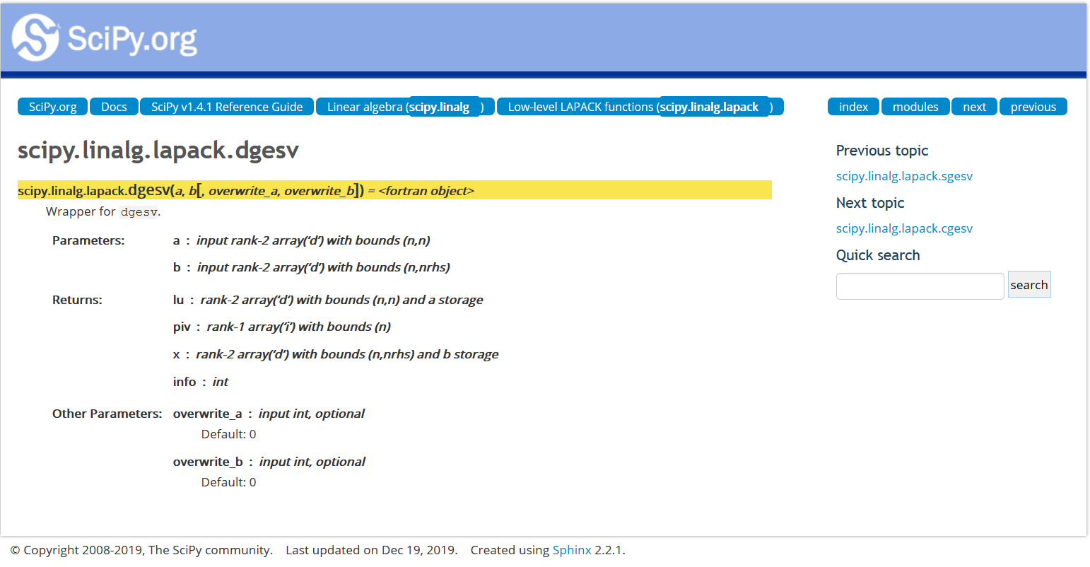
import scipy.linalg.lapack as lapack

printcols(dir(lapack),6)
HAS_ILP64 clartg dgetc2 dtrsyl ssbev zgttrs _DeprecatedImport claswp dgetrf dtrtri ssbevd zhbevd __all__ clauum dgetri dtrtrs ssbevx zhbevx __builtins__ cpbsv dgetri_lwork dtrttf ssfrk zhecon __cached__ cpbtrf dgetrs dtrttp sstebz zheequb __doc__ cpbtrs dgges dtzrzf sstein zheev __file__ cpftrf dggev dtzrzf_lwork sstemr zheev_lwork __loader__ cpftri dgglse flapack sstemr_lwork zheevd __name__ cpftrs dgglse_lwork get_lapack_funcs ssterf zheevd_lwork __package__ cpocon dgtsv ilaver sstev zheevr __spec__ cposv dgtsvx routine ssycon zheevr_lwork _check_work_float cposvx dgttrf sgbsv ssyconv zheevx _clapack cpotrf dgttrs sgbtrf ssyequb zheevx_lwork _compute_lwork cpotri dlamch sgbtrs ssyev zhegst _flapack cpotrs dlange sgebal ssyev_lwork zhegv _flapack_64 cppcon dlarf sgecon ssyevd zhegv_lwork _get_funcs cppsv dlarfg sgeequ ssyevd_lwork zhegvd _int32_max cpptrf dlartg sgeequb ssyevr zhegvx _int64_max cpptri dlasd4 sgees ssyevr_lwork zhegvx_lwork _lapack_alias cpptrs dlaswp sgeev ssyevx zhesv _memoize_get_funcs cpstf2 dlauum sgeev_lwork ssyevx_lwork zhesv_lwork _np cpstrf dorcsd sgehrd ssygst zhesvx cgbsv cpteqr dorcsd_lwork sgehrd_lwork ssygv zhesvx_lwork cgbtrf cptsv dorghr sgejsv ssygv_lwork zhetrd cgbtrs cptsvx dorghr_lwork sgels ssygvd zhetrd_lwork cgebal cpttrf dorgqr sgels_lwork ssygvx zhetrf cgecon cpttrs dorgrq sgelsd ssygvx_lwork zhetrf_lwork cgeequ crot dormqr sgelsd_lwork ssysv zhfrk cgeequb csycon dormrz sgelss ssysv_lwork zlange cgees csyconv dormrz_lwork sgelss_lwork ssysvx zlarf cgeev csyequb dpbsv sgelsy ssysvx_lwork zlarfg cgeev_lwork csysv dpbtrf sgelsy_lwork ssytf2 zlartg cgehrd csysv_lwork dpbtrs sgemqrt ssytrd zlaswp cgehrd_lwork csysvx dpftrf sgeqp3 ssytrd_lwork zlauum cgels csysvx_lwork dpftri sgeqrf ssytrf zpbsv cgels_lwork csytf2 dpftrs sgeqrf_lwork ssytrf_lwork zpbtrf cgelsd csytrf dpocon sgeqrfp stbtrs zpbtrs cgelsd_lwork csytrf_lwork dposv sgeqrfp_lwork stfsm zpftrf cgelss ctbtrs dposvx sgeqrt stfttp zpftri cgelss_lwork ctfsm dpotrf sgerqf stfttr zpftrs cgelsy ctfttp dpotri sgesc2 stgexc zpocon cgelsy_lwork ctfttr dpotrs sgesdd stgsen zposv cgemqrt ctgexc dppcon sgesdd_lwork stgsen_lwork zposvx cgeqp3 ctgsen dppsv sgesv stpmqrt zpotrf cgeqrf ctgsen_lwork dpptrf sgesvd stpqrt zpotri cgeqrf_lwork ctpmqrt dpptri sgesvd_lwork stpttf zpotrs cgeqrfp ctpqrt dpptrs sgesvx stpttr zppcon cgeqrfp_lwork ctpttf dpstf2 sgetc2 strsyl zppsv cgeqrt ctpttr dpstrf sgetrf strtri zpptrf cgerqf ctrsyl dpteqr sgetri strtrs zpptri cgesc2 ctrtri dptsv sgetri_lwork strttf zpptrs cgesdd ctrtrs dptsvx sgetrs strttp zpstf2 cgesdd_lwork ctrttf dpttrf sgges stzrzf zpstrf cgesv ctrttp dpttrs sggev stzrzf_lwork zpteqr cgesvd ctzrzf dsbev sgglse zgbsv zptsv cgesvd_lwork ctzrzf_lwork dsbevd sgglse_lwork zgbtrf zptsvx cgesvx cuncsd dsbevx sgtsv zgbtrs zpttrf cgetc2 cuncsd_lwork dsfrk sgtsvx zgebal zpttrs cgetrf cunghr dstebz sgttrf zgecon zrot cgetri cunghr_lwork dstein sgttrs zgeequ zsycon cgetri_lwork cungqr dstemr slamch zgeequb zsyconv cgetrs cungrq dstemr_lwork slange zgees zsyequb cgges cunmqr dsterf slarf zgeev zsysv cggev cunmrz dstev slarfg zgeev_lwork zsysv_lwork cgglse cunmrz_lwork dsycon slartg zgehrd zsysvx cgglse_lwork dgbsv dsyconv slasd4 zgehrd_lwork zsysvx_lwork cgtsv dgbtrf dsyequb slaswp zgels zsytf2 cgtsvx dgbtrs dsyev slauum zgels_lwork zsytrf cgttrf dgebal dsyev_lwork sorcsd zgelsd zsytrf_lwork cgttrs dgecon dsyevd sorcsd_lwork zgelsd_lwork ztbtrs chbevd dgeequ dsyevd_lwork sorghr zgelss ztfsm chbevx dgeequb dsyevr sorghr_lwork zgelss_lwork ztfttp checon dgees dsyevr_lwork sorgqr zgelsy ztfttr cheequb dgeev dsyevx sorgrq zgelsy_lwork ztgexc cheev dgeev_lwork dsyevx_lwork sormqr zgemqrt ztgsen cheev_lwork dgehrd dsygst sormrz zgeqp3 ztgsen_lwork cheevd dgehrd_lwork dsygv sormrz_lwork zgeqrf ztpmqrt cheevd_lwork dgejsv dsygv_lwork spbsv zgeqrf_lwork ztpqrt cheevr dgels dsygvd spbtrf zgeqrfp ztpttf cheevr_lwork dgels_lwork dsygvx spbtrs zgeqrfp_lwork ztpttr cheevx dgelsd dsygvx_lwork spftrf zgeqrt ztrsyl cheevx_lwork dgelsd_lwork dsysv spftri zgerqf ztrtri chegst dgelss dsysv_lwork spftrs zgesc2 ztrtrs chegv dgelss_lwork dsysvx spocon zgesdd ztrttf chegv_lwork dgelsy dsysvx_lwork sposv zgesdd_lwork ztrttp chegvd dgelsy_lwork dsytf2 sposvx zgesv ztzrzf chegvx dgemqrt dsytrd spotrf zgesvd ztzrzf_lwork chegvx_lwork dgeqp3 dsytrd_lwork spotri zgesvd_lwork zuncsd chesv dgeqrf dsytrf spotrs zgesvx zuncsd_lwork chesv_lwork dgeqrf_lwork dsytrf_lwork sppcon zgetc2 zunghr chesvx dgeqrfp dtbtrs sppsv zgetrf zunghr_lwork chesvx_lwork dgeqrfp_lwork dtfsm spptrf zgetri zungqr chetrd dgeqrt dtfttp spptri zgetri_lwork zungrq chetrd_lwork dgerqf dtfttr spptrs zgetrs zunmqr chetrf dgesc2 dtgexc spstf2 zgges zunmrz chetrf_lwork dgesdd dtgsen spstrf zggev zunmrz_lwork chfrk dgesdd_lwork dtgsen_lwork spteqr zgglse clange dgesv dtpmqrt sptsv zgglse_lwork clapack dgesvd dtpqrt sptsvx zgtsv clarf dgesvd_lwork dtpttf spttrf zgtsvx clarfg dgesvx dtpttr spttrs zgttrf
C++ API
Scipy wrapper API
Eigen
- https://eigen.tuxfamily.org/dox/
- Written in C++
- Previously used for linear algebra in Tensorflow (single CPU variant probably)
- Low and high-level (e.g. matrix decompositions) linear algebra functions
- Sparse linear algebra
- Can use BLAS/LaPACK as a backend https://eigen.tuxfamily.org/dox/TopicUsingBlasLapack.html
...name can be annoyingly google-proof however
Take-home message
Much (most) code you get for free, or even pay for, that implements mathematical algorithms may be of limited value.
Linear algebra, however, is "solved", in terms of numerical programming.
Your main concern is to find an implementation that fits for your application. E.g. parallel, or sparse, or optimized for a particular CPU.
Lab: Import and directly use packages in Python
- BLAS - compute a dot product of two random vectors
- LaPACK - solve a random linear system
II. Overview of leading Python tools
Leading Python tools:
Jupyter - "notebooks" for inline code + LaTex math + markup, etc.
NumPy - low-level array & matrix handling and algorithms
SciPy - higher level numerical algorithms (still fairly basic)
Matplotlib - matlab-style plotting & image display
SkLearn - (Scikit-learn) Machine Learning library
NumPy (short version)
- Numerical algorithm toolbox
- Similar to Matlab but Many key differences, such as zero-based indexing (like C) instead of one-based (like math texts).
- Uses BLAS/LAPACK typically
- NumPy Arrays - special data structure which allows direct and efficient linear algebra manipulations (basically a list with added functionality).
import numpy as np

x = np.array([2,0,1,8])

print(x)
[2 0 1 8]
Fast Numerical Mathematics
l = range(1234)
%timeit [i ** 2 for i in l]
389 µs ± 8.15 µs per loop (mean ± std. dev. of 7 runs, 1000 loops each)
import numpy as np
a = np.arange(1234)
%timeit a ** 2
1.41 µs ± 7.46 ns per loop (mean ± std. dev. of 7 runs, 1000000 loops each)
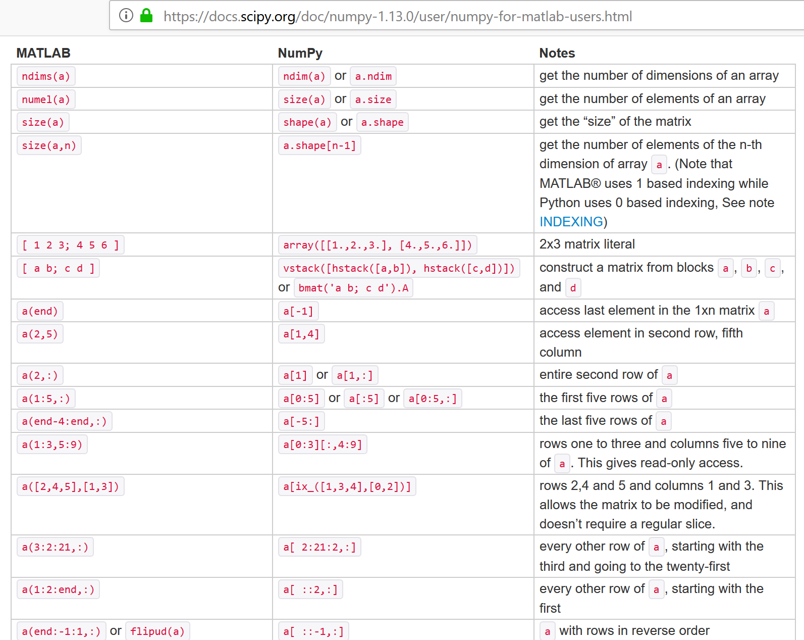
NumPy for Matlab Users
help(np.array)
Help on built-in function array in module numpy.core.multiarray:

array(...)
    array(object, dtype=None, copy=True, order='K', subok=False, ndmin=0)

    Create an array.

    Parameters
    ----------
    object : array_like
        An array, any object exposing the array interface, an object whose
        __array__ method returns an array, or any (nested) sequence.
    dtype : data-type, optional
        The desired data-type for the array.  If not given, then the type will
        be determined as the minimum type required to hold the objects in the
        sequence.  This argument can only be used to 'upcast' the array.  For
        downcasting, use the .astype(t) method.
    copy : bool, optional
        If true (default), then the object is copied.  Otherwise, a copy will
        only be made if __array__ returns a copy, if obj is a nested sequence,
        or if a copy is needed to satisfy any of the other requirements
        (`dtype`, `order`, etc.).
    order : {'K', 'A', 'C', 'F'}, optional
        Specify the memory layout of the array. If object is not an array, the
        newly created array will be in C order (row major) unless 'F' is
        specified, in which case it will be in Fortran order (column major).
        If object is an array the following holds.

        ===== ========= ===================================================
        order  no copy                     copy=True
        ===== ========= ===================================================
        'K'   unchanged F & C order preserved, otherwise most similar order
        'A'   unchanged F order if input is F and not C, otherwise C order
        'C'   C order   C order
        'F'   F order   F order
        ===== ========= ===================================================

        When ``copy=False`` and a copy is made for other reasons, the result is
        the same as if ``copy=True``, with some exceptions for `A`, see the
        Notes section. The default order is 'K'.
    subok : bool, optional
        If True, then sub-classes will be passed-through, otherwise
        the returned array will be forced to be a base-class array (default).
    ndmin : int, optional
        Specifies the minimum number of dimensions that the resulting
        array should have.  Ones will be pre-pended to the shape as
        needed to meet this requirement.

    Returns
    -------
    out : ndarray
        An array object satisfying the specified requirements.

    See Also
    --------
    empty, empty_like, zeros, zeros_like, ones, ones_like, full, full_like

    Notes
    -----
    When order is 'A' and `object` is an array in neither 'C' nor 'F' order,
    and a copy is forced by a change in dtype, then the order of the result is
    not necessarily 'C' as expected. This is likely a bug.

    Examples
    --------
    >>> np.array([1, 2, 3])
    array([1, 2, 3])

    Upcasting:

    >>> np.array([1, 2, 3.0])
    array([ 1.,  2.,  3.])

    More than one dimension:

    >>> np.array([[1, 2], [3, 4]])
    array([[1, 2],
           [3, 4]])

    Minimum dimensions 2:

    >>> np.array([1, 2, 3], ndmin=2)
    array([[1, 2, 3]])

    Type provided:

    >>> np.array([1, 2, 3], dtype=complex)
    array([ 1.+0.j,  2.+0.j,  3.+0.j])

    Data-type consisting of more than one element:

    >>> x = np.array([(1,2),(3,4)],dtype=[('a','<i4'),('b','<i4')])
    >>> x['a']
    array([1, 3])

    Creating an array from sub-classes:

    >>> np.array(np.mat('1 2; 3 4'))
    array([[1, 2],
           [3, 4]])

    >>> np.array(np.mat('1 2; 3 4'), subok=True)
    matrix([[1, 2],
            [3, 4]])
Will cover more later, but first a quick intro to some other packages.
SciPy
Implements higher-level scientific algorithms using NumPy. Examples:
- Integration (scipy.integrate)
- Optimization (scipy.optimize)
- Interpolation (scipy.interpolate)
- Signal Processing (scipy.signal)
- Linear Algebra (scipy.linalg)
- Statistics (scipy.stats)
- File IO (scipy.io)
Also uses BLAS/LAPACK
import scipy
printcols(dir(scipy),2)
LowLevelCallable   ndimage
__numpy_version__  odr
__version__        optimize
cluster            show_config
fft                signal
fftpack            sparse
integrate          spatial
interpolate        special
io                 stats
linalg             test
misc
printcols(dir(scipy.stats))
ConstantInputWarning      bayes_mvs                 gausshyper                matrix_normal             rvs_ratio_uniforms
DegenerateDataWarning     bernoulli                 gaussian_kde              maxwell                   scoreatpercentile
FitError                  beta                      genexpon                  median_abs_deviation      sem
NearConstantInputWarning  betabinom                 genextreme                median_test               semicircular
NumericalInverseHermite   betaprime                 gengamma                  mielke                    shapiro
__all__                   biasedurn                 genhalflogistic           mode                      siegelslopes
__builtins__              binned_statistic          genhyperbolic             moment                    sigmaclip
__cached__                binned_statistic_2d       geninvgauss               monte_carlo_test          skellam
__doc__                   binned_statistic_dd       genlogistic               mood                      skew
__file__                  binom                     gennorm                   morestats                 skewcauchy
__loader__                binom_test                genpareto                 moyal                     skewnorm
__name__                  binomtest                 geom                      mstats                    skewtest
__package__               boltzmann                 gibrat                    mstats_basic              somersd
__path__                  bootstrap                 gilbrat                   mstats_extras             spearmanr
__spec__                  boschloo_exact            gmean                     multinomial               special_ortho_group
_axis_nan_policy          boxcox                    gompertz                  multiscale_graphcorr      statlib
_biasedurn                boxcox_llf                gstd                      multivariate_hypergeom    stats
_binned_statistic         boxcox_normmax            gumbel_l                  multivariate_normal       studentized_range
_binomtest                boxcox_normplot           gumbel_r                  multivariate_t            t
_boost                    bradford                  gzscore                   mvn                       test
_common                   brunnermunzel             halfcauchy                mvsdist                   theilslopes
_constants                burr                      halfgennorm               nakagami                  tiecorrect
_continuous_distns        burr12                    halflogistic              nbinom                    tmax
_crosstab                 cauchy                    halfnorm                  ncf                       tmean
_discrete_distns          chi                       hmean                     nchypergeom_fisher        tmin
_distn_infrastructure     chi2                      hypergeom                 nchypergeom_wallenius     trapezoid
_distr_params             chi2_contingency          hypsecant                 nct                       trapz
_entropy                  chisquare                 invgamma                  ncx2                      triang
_fit                      circmean                  invgauss                  nhypergeom                trim1
_hypotests                circstd                   invweibull                norm                      trim_mean
_hypotests_pythran        circvar                   invwishart                normaltest                trimboth
_kde                      combine_pvalues           iqr                       norminvgauss              truncexpon
_ksstats                  contingency               jarque_bera               obrientransform           truncnorm
_levy_stable              cosine                    johnsonsb                 ortho_group               truncweibull_min
_mannwhitneyu             cramervonmises            johnsonsu                 page_trend_test           tsem
_morestats                cramervonmises_2samp      kappa3                    pareto                    tstd
_mstats_basic             crystalball               kappa4                    pearson3                  ttest_1samp
_mstats_extras            cumfreq                   kde                       pearsonr                  ttest_ind
_multivariate             describe                  kendalltau                percentileofscore         ttest_ind_from_stats
_mvn                      dgamma                    kruskal                   permutation_test          ttest_rel
_page_trend_test          differential_entropy      ks_1samp                  planck                    tukey_hsd
_qmc                      dirichlet                 ks_2samp                  pmean                     tukeylambda
_qmc_cy                   distributions             ksone                     pointbiserialr            tvar
_relative_risk            dlaplace                  kstat                     poisson                   uniform
_resampling               dweibull                  kstatvar                  power_divergence          unitary_group
_rvs_sampling             energy_distance           kstest                    powerlaw                  variation
_sobol                    entropy                   kstwo                     powerlognorm              vonmises
_statlib                  epps_singleton_2samp      kstwobign                 powernorm                 vonmises_line
_stats                    erlang                    kurtosis                  ppcc_max                  wald
_stats_mstats_common      expon                     kurtosistest              ppcc_plot                 wasserstein_distance
_stats_py                 exponnorm                 laplace                   probplot                  weibull_max
_tukeylambda_stats        exponpow                  laplace_asymmetric        qmc                       weibull_min
_unuran                   exponweib                 levene                    randint                   weightedtau
_variation                f                         levy                      random_correlation        wilcoxon
_warnings_errors          f_oneway                  levy_l                    rankdata                  wishart
alexandergovern           fatiguelife               levy_stable               ranksums                  wrapcauchy
alpha                     find_repeats              linregress                rayleigh                  yeojohnson
anderson                  fisher_exact              loggamma                  rdist                     yeojohnson_llf
anderson_ksamp            fisk                      logistic                  recipinvgauss             yeojohnson_normmax
anglit                    fit                       loglaplace                reciprocal                yeojohnson_normplot
ansari                    fligner                   lognorm                   relfreq                   yulesimon
arcsine                   foldcauchy                logser                    rice                      zipf
argus                     foldnorm                  loguniform                rv_continuous             zipfian
barnard_exact             friedmanchisquare         lomax                     rv_discrete               zmap
bartlett                  gamma                     mannwhitneyu              rv_histogram              zscore
Matplotlib
Tutorial from: https://github.com/amueller/scipy-2017-sklearn/blob/master/notebooks/02.Scientific_Computing_Tools_in_Python.ipynb
Another important part of machine learning is the visualization of data. The most common
tool for this in Python is matplotlib. It is an extremely flexible package, and
we will go over some basics here.
Jupyter has built-in "magic functions", the "matoplotlib inline" mode, which will draw the plots directly inside the notebook. Should be on by default.
%matplotlib inline

import matplotlib.pyplot as plt

# Plotting a line
x = np.linspace(0, 10, 100)
plt.plot(x, np.sin(x));

# Scatter-plot points
x = np.random.normal(size=500)
y = np.random.normal(size=500)
plt.scatter(x, y);

# Showing images using imshow
# - note that origin is at the top-left by default!

#x = np.linspace(1, 12, 100)
#y = x[:, np.newaxis]
#im = y * np.sin(x) * np.cos(y)
im = np.array([[1, 2, 3],[4,5,6],[6,7,8]])
import matplotlib.pyplot as plt

plt.imshow(im);
plt.colorbar();
plt.xlabel('x')
plt.ylabel('y')
plt.show();

# Contour plots
# - note that origin here is at the bottom-left by default!
plt.contour(im);

# 3D plotting
from mpl_toolkits.mplot3d import Axes3D
ax = plt.axes(projection='3d')
xgrid, ygrid = np.meshgrid(x, y.ravel())
ax.plot_surface(xgrid, ygrid, im, cmap=plt.cm.viridis, cstride=2, rstride=2, linewidth=0);

There are many more plot types available. See matplotlib gallery.
Test these examples: copy the Source Code
link, and put it in a notebook using the %load magic.
For example:
# %load http://matplotlib.org/mpl_examples/pylab_examples/ellipse_collection.py
SkLearn
Many Machine Learning functions.
Couple dozen core developers + hundreds of other contributors.
2011 tutorial has over 10,000 citations.
"Scikit-learn: Machine Learning in Python", Fabian Pedregosa, Gaël Varoquaux, Alexandre Gramfort, Vincent Michel, Bertrand Thirion, Olivier Grisel, Mathieu Blondel, Peter Prettenhofer, Ron Weiss, Vincent Dubourg, Jake Vanderplas, Alexandre Passos, David Cournapeau, Matthieu Brucher, Matthieu Perrot, Édouard Duchesnay; 12(Oct):2825−2830, 2011
Considered leading Machine Learning toolbox. Was getting discarded as field switched from sinlge CPU to multicore, but appears to be making comeback with parallel upgrades
# conda install anaconda::scikit-learn

import sklearn as sk

printcols(dir(sk),2)
__SKLEARN_SETUP__  base
__all__            clone
__builtins__       config_context
__cached__         exceptions
__check_build      externals
__doc__            get_config
__file__           logger
__loader__         logging
__name__           os
__package__        random
__path__           set_config
__spec__           setup_module
__version__        show_versions
_config            sys
_distributor_init  utils
printcols(dir(sk.base),2)
BaseEstimator            _check_feature_names_in
BiclusterMixin           _check_y
ClassifierMixin          _get_feature_names
ClusterMixin             _is_pairwise
DensityMixin             _num_features
MetaEstimatorMixin       _pprint
MultiOutputMixin         _safe_tags
OutlierMixin             check_X_y
RegressorMixin           check_array
TransformerMixin         clone
_DEFAULT_TAGS            copy
_IS_32BIT                defaultdict
_OneToOneFeatureMixin    estimator_html_repr
_UnstableArchMixin       get_config
__builtins__             inspect
__cached__               is_classifier
__doc__                  is_outlier_detector
__file__                 is_regressor
__loader__               np
__name__                 platform
__package__              re
__spec__                 warnings
__version__
Machine Learning Framework using Sklearn
Given training data $(\mathbf x_{(i)},y_i)$ for $i=1,...,m$ --> lists of samples $\verb|X|$ and labels $\verb|y|$
Choose a model $f(\cdot)$ where we want to make $f(\mathbf x_{(i)})\approx y_i$ (for all $i$) --> choose sklearn estimator to use
Define a loss function $L(f(\mathbf x), y)$ to minimize by changing $f(\cdot)$ ...by adjusting the weights --> default choises for estimators, sometimes multiple options
The Sklearn API
sklearn has an Object Oriented interface
Most models/transforms/objects in sklearn are Estimator objects
class Estimator(object):

    def fit(self, X, y=None):
        """Fit model to data X (and y)"""
        self.some_attribute = self.some_fitting_method(X, y)
        return self

    def predict(self, X_test):
        """Make prediction based on passed features"""
        pred = self.make_prediction(X_test)
        return pred

model = Estimator()
The Estimator class defines a fit() method as well as a predict() method. For an instance of an Estimator stored in a variable model:
model.fit: fits the model with the passed in training data. For supervised models, it also accepts a second argumentythat corresponds to the labels (model.fit(X, y). For unsupervised models, there are no labels so you only need to pass in the feature matrix (model.fit(X))Since the interface is very OO, the instance itself stores the results of the
fitinternally. And as such you must alwaysfit()before youpredict()on the same object.model.predict: predicts new labels for any new datapoints passed in (model.predict(X_test)) and returns an array equal in length to the number of rows of what is passed in containing the predicted labels.
Types of subclass of estimator:
- Supervised
- Unsupervised
- Feature Processing
Supervised
Supervised estimators in addition to the above methods typically also have:
model.predict_proba: For classifiers that have a notion of probability (or some measure of confidence in a prediction) this method returns those "probabilities". The label with the highest probability is what is returned by themodel.predict()` mehod from above.model.score: For both classification and regression models, this method returns some measure of validation of the model (which is configurable). For example, in regression the default is typically R^2 and classification it is accuracy.
Unsupervised - Transformer interface
Some estimators in the library implement this.
Unsupervised in this case refers to any method that does not need labels, including unsupervised classifiers, preprocessing (like tf-idf), dimensionality reduction, etc.
The transformer interface usually defines two additional methods:
model.transform: Given an unsupervised model, transform the input into a new basis (or feature space). This accepts on argument (usually a feature matrix) and returns a matrix of the input transformed. Note: You need tofit()the model before you transform it.model.fit_transform: For some models you may not need tofit()andtransform()separately. In these cases it is more convenient to do both at the same time.
X = [[0], [1], [2], [3]]
y = [0, 0, 1, 1]
from sklearn.neighbors import KNeighborsClassifier
neigh = KNeighborsClassifier(n_neighbors=3)
neigh.fit(X, y)
print(neigh.predict([[1.1]]))
print(neigh.predict_proba([[0.9]]))
[0]
[[0.66666667 0.33333333]]
Recap
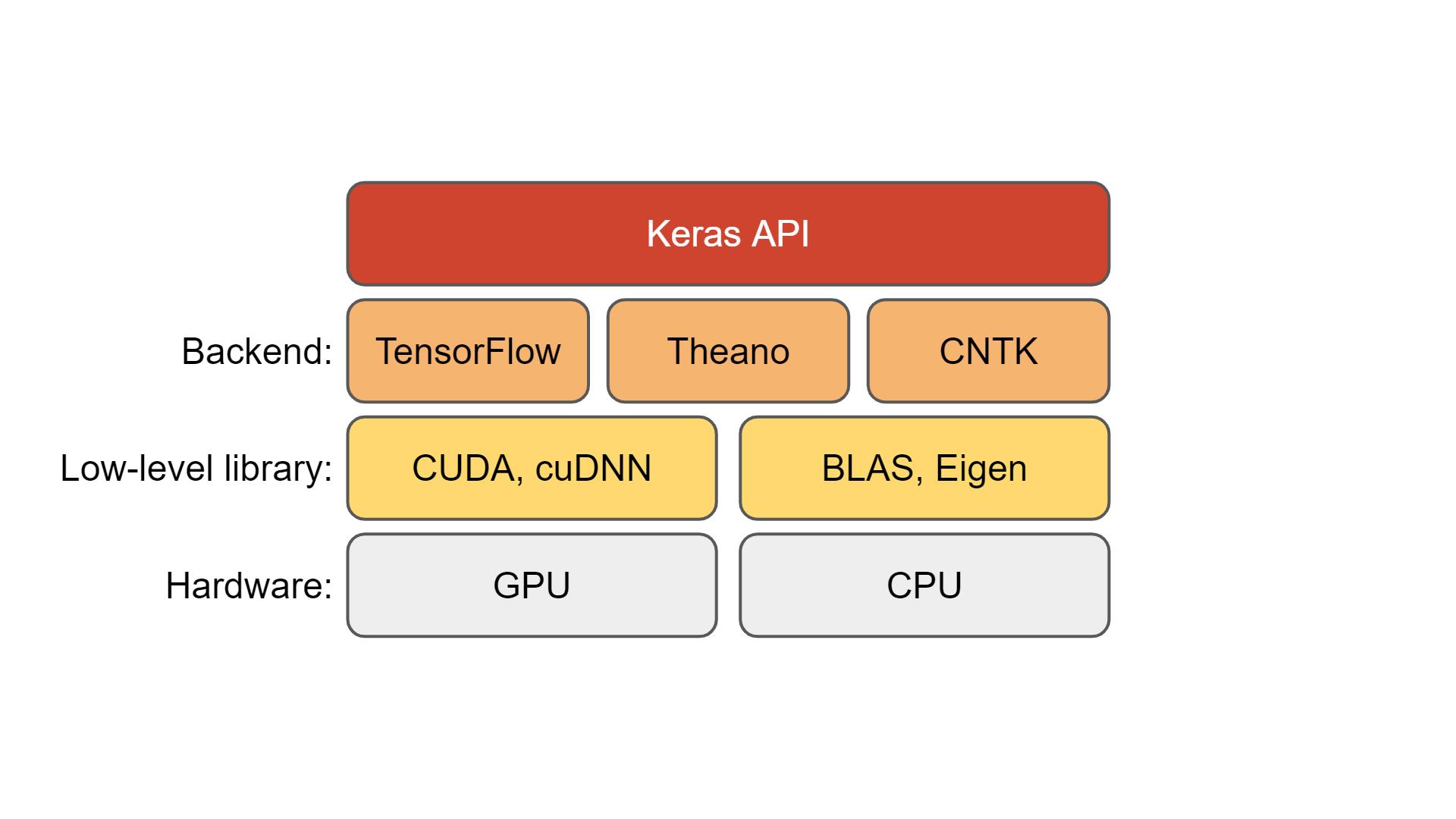
- Mathematical software is implemented hierarchically
- BLAS = Lowest level(s), implemented on particular hardware, e.g. for SIMD processors
- Higher level functions (solvers and decompositions) calls BLAS to implement internal computations
- Structured and Sparse matrix libraries also call BLAS typically (convert large sparse problems to small dense problems)
- Modern alternatives also can utilize BLAS/LAPACK backend and also suppot hardware-specific replacements (e.g. CUDA)
IV. NumPy Basics
NumPy Arrays for Vectors
x = np.array([2,0,1,8])

x
array([2, 0, 1, 8])
NumPy arrays are zero-based like Python lists
print(x[0],x[3])
2 8
Matlab-ish slicing
A = np.array([[1,2,3],[4,5,6],[7,8,9]])
print(A)
[[1 2 3]
 [4 5 6]
 [7 8 9]]
print(A[:,0])
[1 4 7]
print(A[1,:])
[4 5 6]
print(A[1,1:])
[5 6]
$\verb|numpy.linalg|$
- Use BLAS and LAPACK to provide efficient low level implementations of standard linear algebra algorithms.
- Those libraries may be provided by NumPy itself using C versions of a subset of their reference implementations
- When possible, highly optimized libraries that take advantage of specialized processor functionality are preferred.
- Examples of such libraries are OpenBLAS, MKL (TM), and ATLAS.
https://docs.scipy.org/doc/numpy/reference/routines.linalg.html
Matrix and vector products
- dot(a, b[, out]) Dot product of two arrays.
- linalg.multi_dot(arrays) Compute the dot product of two or more arrays in a single function call, while automatically selecting the fastest evaluation order.
- vdot(a, b) Return the dot product of two vectors.
- inner(a, b) Inner product of two arrays.
- outer(a, b[, out]) Compute the outer product of two vectors.
- matmul(x1, x2, /[, out, casting, order, …]) Matrix product of two arrays.
- tensordot(a, b[, axes]) Compute tensor dot product along specified axes.
- einsum(subscripts, *operands[, out, dtype, …]) Evaluates the Einstein summation convention on the operands.
- einsum_path(subscripts, *operands[, optimize]) Evaluates the lowest cost contraction order for an einsum expression by considering the creation of intermediate arrays.
- linalg.matrix_power(a, n) Raise a square matrix to the (integer) power n.
- kron(a, b) Kronecker product of two arrays.
Decompositions
- linalg.cholesky(a) Cholesky decomposition.
- linalg.qr(a[, mode]) Compute the qr factorization of a matrix.
- linalg.svd(a[, full_matrices, compute_uv, …]) Singular Value Decomposition.
Matrix eigenvalues
- linalg.eig(a) Compute the eigenvalues and right eigenvectors of a square array.
- linalg.eigh(a[, UPLO]) Return the eigenvalues and eigenvectors of a complex Hermitian (conjugate symmetric) or a real symmetric matrix.
- linalg.eigvals(a) Compute the eigenvalues of a general matrix.
- linalg.eigvalsh(a[, UPLO]) Compute the eigenvalues of a complex Hermitian or real symmetric matrix.
Norms and other numbers
- linalg.norm(x[, ord, axis, keepdims]) Matrix or vector norm.
- linalg.cond(x[, p]) Compute the condition number of a matrix.
- linalg.det(a) Compute the determinant of an array.
- linalg.matrix_rank(M[, tol, hermitian]) Return matrix rank of array using SVD method
- linalg.slogdet(a) Compute the sign and (natural) logarithm of the determinant of an array.
- trace(a[, offset, axis1, axis2, dtype, out]) Return the sum along diagonals of the array.
Solving equations and inverting matrices
- linalg.solve(a, b) Solve a linear matrix equation, or system of linear scalar equations.
- linalg.tensorsolve(a, b[, axes]) Solve the tensor equation a x = b for x.
- linalg.lstsq(a, b[, rcond]) Return the least-squares solution to a linear matrix equation.
- linalg.inv(a) Compute the (multiplicative) inverse of a matrix.
- linalg.pinv(a[, rcond, hermitian]) Compute the (Moore-Penrose) pseudo-inverse of a matrix.
- linalg.tensorinv(a[, ind]) Compute the ‘inverse’ of an N-dimensional array.
"Vectorization"
Converting loops into linear algebra functions where loop is performed at lower level
E.g. instead of looping over a list to compute squares of elements, make into array and "square" array
v = [1,2,3,4,5]

v2 = []
for v_k in v:
    v2.append(v_k**2)
v2
[1, 4, 9, 16, 25]
np.array(v)**2
array([ 1, 4, 9, 16, 25], dtype=int32)
Dot Product using NumPy
w = np.array([1, 2])
v = np.array([3, 4])
np.dot(w,v)
11
w = np.array([0, 1])
v = np.array([1, 0])
np.dot(w,v)
0
w = np.array([1, 2])
v = np.array([-2, 1])
np.dot(w,v)
0
Matrix-vector multiplication using NumPy - CAUTION
NumPy implements a broadcast version of multiplication when using the "*" operator.
It guesses what you mean rather by seeking ways the shapes match, rather than giving error.
w = np.array([[2,-6],[-1, 4]])
v = np.array([12,46])

w*v
array([[  24, -276],
       [ -12,  184]])
v+w
array([[14, 40],
       [11, 50]])
"Broadcasting"
Multiply matrices or vectrors in an element-wise manner by repeating "singular" dimensions.
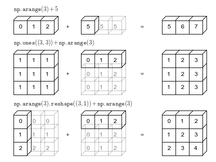
Matlab and Numpy automatically do this now.
Also (and previously) in matlab, e.g.: "brcm(@plus, A, x). numpy.broadcast
For true "Matrix-vector" multiplication, use matmul or "@"
a special case of matrix-matrix multiplication
w = np.array([[ 2, -6],
              [-1,  4]])
v = np.array([[+1],
              [-1]])
np.matmul(w,v)
array([[ 8],
       [-5]])
w@v
array([ 8, -5])
Matrix-matrix multiplication
A = np.array([[1,2],[3, 4]])
B = np.array([[1,0],[1, 1]])
A*B
array([[1, 0],
       [3, 4]])
What is this doing?
np.matmul(A,B)
array([[3, 2],
       [7, 4]])
np.dot(A,B)
array([[3, 2],
       [7, 4]])
A@B
array([[3, 2],
       [7, 4]])
u = [1,2]
v = [1,3]
np.dot(np.array(u),np.array(v))
7
Reshaping vectors into matrices and whatever else you want
x = np.array([1,2,3,4])
x = x.reshape(4,1)
print(x.reshape(4,1))
[[1]
 [2]
 [3]
 [4]]
print(x.reshape(2,2))
[[1 2]
 [3 4]]
print(x)
x_T = x.transpose()
print (x_T)
print (x_T.shape)
print(x.T)
[[1]
 [2]
 [3]
 [4]]
[[1 2 3 4]]
(1, 4)
[[1 2 3 4]]
Famous matrices in NumPy
np.zeros((3,4))
array([[0., 0., 0., 0.],
       [0., 0., 0., 0.],
       [0., 0., 0., 0.]])
np.ones((3,4))
array([[1., 1., 1., 1.],
       [1., 1., 1., 1.],
       [1., 1., 1., 1.]])
np.eye(3)
array([[1., 0., 0.],
       [0., 1., 0.],
       [0., 0., 1.]])
D = np.diag([1,2,3])
print(D)
[[1 0 0]
 [0 2 0]
 [0 0 3]]
np.diag(D)
array([1, 2, 3])
np.random.rand(3,4) # note two inputs, not tuple
array([[0.99147344, 0.01075122, 0.81974321, 0.10942128],
       [0.94041317, 0.50408574, 0.71896232, 0.12113072],
       [0.77483078, 0.32627551, 0.44489225, 0.13208849]])
np.random.randn(3,4)
array([[ 1.09642959,  1.40715723, -0.30932909,  0.66846735],
       [ 0.22536484, -0.08283707, -0.60713286, -0.16836462],
       [-1.20191307,  1.53390883, -0.48587343, -0.84379159]])
NumPy Inverse
A = np.array([[1,2],[4,5]])
iA = np.linalg.inv(A)
print(iA)
print(np.matmul(A,iA))
[[-1.66666667  0.66666667]
 [ 1.33333333 -0.33333333]]
[[1. 0.]
 [0. 1.]]
2.*8.
16.0
A = np.random.randint(0, 10, size=(3, 3))
A_inv = np.linalg.inv(A)
print(A)
print(A_inv)
print(np.matmul(A,A_inv))
[[2 6 4]
 [5 7 1]
 [5 3 2]]
[[-1.25000000e-01 -1.11022302e-17  2.50000000e-01]
 [ 5.68181818e-02  1.81818182e-01 -2.04545455e-01]
 [ 2.27272727e-01 -2.72727273e-01  1.81818182e-01]]
[[ 1.00000000e+00  0.00000000e+00 -1.11022302e-16]
 [-2.77555756e-17  1.00000000e+00 -8.32667268e-17]
 [-5.55111512e-17  0.00000000e+00  1.00000000e+00]]
Note that "hard zeros" rarely exist in real world due to limited numerical precision.
Eigenvalue Decomposition in NumPy
A = np.asarray([[.3,.1,.6],[.1,.3,.6],[.15,.15,.70]])

np.linalg.eig(A)
(array([1. , 0.2, 0.1]),
 array([[-5.77350269e-01, -7.07106781e-01, -6.66666667e-01],
        [-5.77350269e-01,  7.07106781e-01, -6.66666667e-01],
        [-5.77350269e-01, -2.74027523e-16,  3.33333333e-01]]))
Note there's only one return
(u,s) = np.linalg.eig(A)
print(u)
print(s)
[1.  0.2 0.1]
[[-5.77350269e-01 -7.07106781e-01 -6.66666667e-01]
 [-5.77350269e-01  7.07106781e-01 -6.66666667e-01]
 [-5.77350269e-01 -2.74027523e-16  3.33333333e-01]]
help(np.linalg.eig)
Help on function eig in module numpy.linalg.linalg:

eig(a)
    Compute the eigenvalues and right eigenvectors of a square array.

    Parameters
    ----------
    a : (..., M, M) array
        Matrices for which the eigenvalues and right eigenvectors will
        be computed

    Returns
    -------
    w : (..., M) array
        The eigenvalues, each repeated according to its multiplicity.
        The eigenvalues are not necessarily ordered. The resulting
        array will be of complex type, unless the imaginary part is
        zero in which case it will be cast to a real type. When `a`
        is real the resulting eigenvalues will be real (0 imaginary
        part) or occur in conjugate pairs

    v : (..., M, M) array
        The normalized (unit "length") eigenvectors, such that the
        column ``v[:,i]`` is the eigenvector corresponding to the
        eigenvalue ``w[i]``.

    Raises
    ------
    LinAlgError
        If the eigenvalue computation does not converge.

    See Also
    --------
    eigvals : eigenvalues of a non-symmetric array.

    eigh : eigenvalues and eigenvectors of a symmetric or Hermitian
           (conjugate symmetric) array.

    eigvalsh : eigenvalues of a symmetric or Hermitian (conjugate symmetric)
               array.

    Notes
    -----

    .. versionadded:: 1.8.0

    Broadcasting rules apply, see the `numpy.linalg` documentation for
    details.

    This is implemented using the _geev LAPACK routines which compute
    the eigenvalues and eigenvectors of general square arrays.

    The number `w` is an eigenvalue of `a` if there exists a vector
    `v` such that ``dot(a,v) = w * v``. Thus, the arrays `a`, `w`, and
    `v` satisfy the equations ``dot(a[:,:], v[:,i]) = w[i] * v[:,i]``
    for :math:`i \in \{0,...,M-1\}`.

    The array `v` of eigenvectors may not be of maximum rank, that is, some
    of the columns may be linearly dependent, although round-off error may
    obscure that fact. If the eigenvalues are all different, then theoretically
    the eigenvectors are linearly independent. Likewise, the (complex-valued)
    matrix of eigenvectors `v` is unitary if the matrix `a` is normal, i.e.,
    if ``dot(a, a.H) = dot(a.H, a)``, where `a.H` denotes the conjugate
    transpose of `a`.

    Finally, it is emphasized that `v` consists of the *right* (as in
    right-hand side) eigenvectors of `a`.  A vector `y` satisfying
    ``dot(y.T, a) = z * y.T`` for some number `z` is called a *left*
    eigenvector of `a`, and, in general, the left and right eigenvectors
    of a matrix are not necessarily the (perhaps conjugate) transposes
    of each other.

    References
    ----------
    G. Strang, *Linear Algebra and Its Applications*, 2nd Ed., Orlando, FL,
    Academic Press, Inc., 1980, Various pp.

    Examples
    --------
    >>> from numpy import linalg as LA

    (Almost) trivial example with real e-values and e-vectors.

    >>> w, v = LA.eig(np.diag((1, 2, 3)))
    >>> w; v
    array([ 1.,  2.,  3.])
    array([[ 1.,  0.,  0.],
           [ 0.,  1.,  0.],
           [ 0.,  0.,  1.]])

    Real matrix possessing complex e-values and e-vectors; note that the
    e-values are complex conjugates of each other.

    >>> w, v = LA.eig(np.array([[1, -1], [1, 1]]))
    >>> w; v
    array([ 1. + 1.j,  1. - 1.j])
    array([[ 0.70710678+0.j        ,  0.70710678+0.j        ],
           [ 0.00000000-0.70710678j,  0.00000000+0.70710678j]])

    Complex-valued matrix with real e-values (but complex-valued e-vectors);
    note that a.conj().T = a, i.e., a is Hermitian.

    >>> a = np.array([[1, 1j], [-1j, 1]])
    >>> w, v = LA.eig(a)
    >>> w; v
    array([  2.00000000e+00+0.j,   5.98651912e-36+0.j]) # i.e., {2, 0}
    array([[ 0.00000000+0.70710678j,  0.70710678+0.j        ],
           [ 0.70710678+0.j        ,  0.00000000+0.70710678j]])

    Be careful about round-off error!

    >>> a = np.array([[1 + 1e-9, 0], [0, 1 - 1e-9]])
    >>> # Theor. e-values are 1 +/- 1e-9
    >>> w, v = LA.eig(a)
    >>> w; v
    array([ 1.,  1.])
    array([[ 1.,  0.],
           [ 0.,  1.]])
SVD in NumPy
np.linalg.svd(A)
(array([[-0.32453643, -0.9458732 ],
        [-0.9458732 ,  0.32453643]]),
 array([6.76782894, 0.44327362]),
 array([[-0.60699365, -0.79470668],
        [ 0.79470668, -0.60699365]]))
Note outputs are U, S, and V-transposed
help(np.linalg.svd)
Help on function svd in module numpy.linalg.linalg:

svd(a, full_matrices=True, compute_uv=True)
    Singular Value Decomposition.

    When `a` is a 2D array, it is factorized as ``u @ np.diag(s) @ vh
    = (u * s) @ vh``, where `u` and `vh` are 2D unitary arrays and `s` is a 1D
    array of `a`'s singular values. When `a` is higher-dimensional, SVD is
    applied in stacked mode as explained below.

    Parameters
    ----------
    a : (..., M, N) array_like
        A real or complex array with ``a.ndim >= 2``.
    full_matrices : bool, optional
        If True (default), `u` and `vh` have the shapes ``(..., M, M)`` and
        ``(..., N, N)``, respectively.  Otherwise, the shapes are
        ``(..., M, K)`` and ``(..., K, N)``, respectively, where
        ``K = min(M, N)``.
    compute_uv : bool, optional
        Whether or not to compute `u` and `vh` in addition to `s`.  True
        by default.

    Returns
    -------
    u : { (..., M, M), (..., M, K) } array
        Unitary array(s). The first ``a.ndim - 2`` dimensions have the same
        size as those of the input `a`. The size of the last two dimensions
        depends on the value of `full_matrices`. Only returned when
        `compute_uv` is True.
    s : (..., K) array
        Vector(s) with the singular values, within each vector sorted in
        descending order. The first ``a.ndim - 2`` dimensions have the same
        size as those of the input `a`.
    vh : { (..., N, N), (..., K, N) } array
        Unitary array(s). The first ``a.ndim - 2`` dimensions have the same
        size as those of the input `a`. The size of the last two dimensions
        depends on the value of `full_matrices`. Only returned when
        `compute_uv` is True.

    Raises
    ------
    LinAlgError
        If SVD computation does not converge.

    Notes
    -----

    .. versionchanged:: 1.8.0
       Broadcasting rules apply, see the `numpy.linalg` documentation for
       details.

    The decomposition is performed using LAPACK routine ``_gesdd``.

    SVD is usually described for the factorization of a 2D matrix :math:`A`.
    The higher-dimensional case will be discussed below. In the 2D case, SVD is
    written as :math:`A = U S V^H`, where :math:`A = a`, :math:`U= u`,
    :math:`S= \mathtt{np.diag}(s)` and :math:`V^H = vh`. The 1D array `s`
    contains the singular values of `a` and `u` and `vh` are unitary. The rows
    of `vh` are the eigenvectors of :math:`A^H A` and the columns of `u` are
    the eigenvectors of :math:`A A^H`. In both cases the corresponding
    (possibly non-zero) eigenvalues are given by ``s**2``.

    If `a` has more than two dimensions, then broadcasting rules apply, as
    explained in :ref:`routines.linalg-broadcasting`. This means that SVD is
    working in "stacked" mode: it iterates over all indices of the first
    ``a.ndim - 2`` dimensions and for each combination SVD is applied to the
    last two indices. The matrix `a` can be reconstructed from the
    decomposition with either ``(u * s[..., None, :]) @ vh`` or
    ``u @ (s[..., None] * vh)``. (The ``@`` operator can be replaced by the
    function ``np.matmul`` for python versions below 3.5.)

    If `a` is a ``matrix`` object (as opposed to an ``ndarray``), then so are
    all the return values.

    Examples
    --------
    >>> a = np.random.randn(9, 6) + 1j*np.random.randn(9, 6)
    >>> b = np.random.randn(2, 7, 8, 3) + 1j*np.random.randn(2, 7, 8, 3)

    Reconstruction based on full SVD, 2D case:

    >>> u, s, vh = np.linalg.svd(a, full_matrices=True)
    >>> u.shape, s.shape, vh.shape
    ((9, 9), (6,), (6, 6))
    >>> np.allclose(a, np.dot(u[:, :6] * s, vh))
    True
    >>> smat = np.zeros((9, 6), dtype=complex)
    >>> smat[:6, :6] = np.diag(s)
    >>> np.allclose(a, np.dot(u, np.dot(smat, vh)))
    True

    Reconstruction based on reduced SVD, 2D case:

    >>> u, s, vh = np.linalg.svd(a, full_matrices=False)
    >>> u.shape, s.shape, vh.shape
    ((9, 6), (6,), (6, 6))
    >>> np.allclose(a, np.dot(u * s, vh))
    True
    >>> smat = np.diag(s)
    >>> np.allclose(a, np.dot(u, np.dot(smat, vh)))
    True

    Reconstruction based on full SVD, 4D case:

    >>> u, s, vh = np.linalg.svd(b, full_matrices=True)
    >>> u.shape, s.shape, vh.shape
    ((2, 7, 8, 8), (2, 7, 3), (2, 7, 3, 3))
    >>> np.allclose(b, np.matmul(u[..., :3] * s[..., None, :], vh))
    True
    >>> np.allclose(b, np.matmul(u[..., :3], s[..., None] * vh))
    True

    Reconstruction based on reduced SVD, 4D case:

    >>> u, s, vh = np.linalg.svd(b, full_matrices=False)
    >>> u.shape, s.shape, vh.shape
    ((2, 7, 8, 3), (2, 7, 3), (2, 7, 3, 3))
    >>> np.allclose(b, np.matmul(u * s[..., None, :], vh))
    True
    >>> np.allclose(b, np.matmul(u, s[..., None] * vh))
    True
QR in NumPy
Q,R = np.linalg.qr(A)
print(Q)
#print(R)
[[-0.85714286  0.39439831 -0.33129458]
 [-0.28571429 -0.89922814 -0.33129458]
 [-0.42857143 -0.18931119  0.88345221]]
np.dot(Q[:,2],Q[:,2])
1.0
Q.T@Q
array([[ 1.00000000e+00,  3.25682983e-17, -6.47535828e-17],
       [ 3.25682983e-17,  1.00000000e+00,  1.03449228e-16],
       [-6.47535828e-17,  1.03449228e-16,  1.00000000e+00]])
help(np.linalg.qr)
Help on function qr in module numpy.linalg.linalg:

qr(a, mode='reduced')
    Compute the qr factorization of a matrix.

    Factor the matrix `a` as *qr*, where `q` is orthonormal and `r` is
    upper-triangular.

    Parameters
    ----------
    a : array_like, shape (M, N)
        Matrix to be factored.
    mode : {'reduced', 'complete', 'r', 'raw', 'full', 'economic'}, optional
        If K = min(M, N), then

        * 'reduced'  : returns q, r with dimensions (M, K), (K, N) (default)
        * 'complete' : returns q, r with dimensions (M, M), (M, N)
        * 'r'        : returns r only with dimensions (K, N)
        * 'raw'      : returns h, tau with dimensions (N, M), (K,)
        * 'full'     : alias of 'reduced', deprecated
        * 'economic' : returns h from 'raw', deprecated.

        The options 'reduced', 'complete, and 'raw' are new in numpy 1.8,
        see the notes for more information. The default is 'reduced', and to
        maintain backward compatibility with earlier versions of numpy both
        it and the old default 'full' can be omitted. Note that array h
        returned in 'raw' mode is transposed for calling Fortran. The
        'economic' mode is deprecated.  The modes 'full' and 'economic' may
        be passed using only the first letter for backwards compatibility,
        but all others must be spelled out. See the Notes for more
        explanation.


    Returns
    -------
    q : ndarray of float or complex, optional
        A matrix with orthonormal columns. When mode = 'complete' the
        result is an orthogonal/unitary matrix depending on whether or not
        a is real/complex. The determinant may be either +/- 1 in that
        case.
    r : ndarray of float or complex, optional
        The upper-triangular matrix.
    (h, tau) : ndarrays of np.double or np.cdouble, optional
        The array h contains the Householder reflectors that generate q
        along with r. The tau array contains scaling factors for the
        reflectors. In the deprecated  'economic' mode only h is returned.

    Raises
    ------
    LinAlgError
        If factoring fails.

    Notes
    -----
    This is an interface to the LAPACK routines dgeqrf, zgeqrf,
    dorgqr, and zungqr.

    For more information on the qr factorization, see for example:
    http://en.wikipedia.org/wiki/QR_factorization

    Subclasses of `ndarray` are preserved except for the 'raw' mode. So if
    `a` is of type `matrix`, all the return values will be matrices too.

    New 'reduced', 'complete', and 'raw' options for mode were added in
    NumPy 1.8.0 and the old option 'full' was made an alias of 'reduced'.  In
    addition the options 'full' and 'economic' were deprecated.  Because
    'full' was the previous default and 'reduced' is the new default,
    backward compatibility can be maintained by letting `mode` default.
    The 'raw' option was added so that LAPACK routines that can multiply
    arrays by q using the Householder reflectors can be used. Note that in
    this case the returned arrays are of type np.double or np.cdouble and
    the h array is transposed to be FORTRAN compatible.  No routines using
    the 'raw' return are currently exposed by numpy, but some are available
    in lapack_lite and just await the necessary work.

    Examples
    --------
    >>> a = np.random.randn(9, 6)
    >>> q, r = np.linalg.qr(a)
    >>> np.allclose(a, np.dot(q, r))  # a does equal qr
    True
    >>> r2 = np.linalg.qr(a, mode='r')
    >>> r3 = np.linalg.qr(a, mode='economic')
    >>> np.allclose(r, r2)  # mode='r' returns the same r as mode='full'
    True
    >>> # But only triu parts are guaranteed equal when mode='economic'
    >>> np.allclose(r, np.triu(r3[:6,:6], k=0))
    True

    Example illustrating a common use of `qr`: solving of least squares
    problems

    What are the least-squares-best `m` and `y0` in ``y = y0 + mx`` for
    the following data: {(0,1), (1,0), (1,2), (2,1)}. (Graph the points
    and you'll see that it should be y0 = 0, m = 1.)  The answer is provided
    by solving the over-determined matrix equation ``Ax = b``, where::

      A = array([[0, 1], [1, 1], [1, 1], [2, 1]])
      x = array([[y0], [m]])
      b = array([[1], [0], [2], [1]])

    If A = qr such that q is orthonormal (which is always possible via
    Gram-Schmidt), then ``x = inv(r) * (q.T) * b``.  (In numpy practice,
    however, we simply use `lstsq`.)

    >>> A = np.array([[0, 1], [1, 1], [1, 1], [2, 1]])
    >>> A
    array([[0, 1],
           [1, 1],
           [1, 1],
           [2, 1]])
    >>> b = np.array([1, 0, 2, 1])
    >>> q, r = LA.qr(A)
    >>> p = np.dot(q.T, b)
    >>> np.dot(LA.inv(r), p)
    array([  1.1e-16,   1.0e+00])
Lab: Least-squares regression various ways
Load Boston house prices dataset.
Formulate linear system and try using inverse and pseudoinverse to solve.
from sklearn.datasets import load_boston
boston = load_boston()
print(dir(boston))
print(boston.data.shape)
print(boston.feature_names)
print(boston.DESCR)
['DESCR', 'data', 'feature_names', 'filename', 'target']
(506, 13)
['CRIM' 'ZN' 'INDUS' 'CHAS' 'NOX' 'RM' 'AGE' 'DIS' 'RAD' 'TAX' 'PTRATIO'
 'B' 'LSTAT']
.. _boston_dataset:

Boston house prices dataset
---------------------------

**Data Set Characteristics:**

    :Number of Instances: 506

    :Number of Attributes: 13 numeric/categorical predictive. Median Value (attribute 14) is usually the target.

    :Attribute Information (in order):
        - CRIM     per capita crime rate by town
        - ZN       proportion of residential land zoned for lots over 25,000 sq.ft.
        - INDUS    proportion of non-retail business acres per town
        - CHAS     Charles River dummy variable (= 1 if tract bounds river; 0 otherwise)
        - NOX      nitric oxides concentration (parts per 10 million)
        - RM       average number of rooms per dwelling
        - AGE      proportion of owner-occupied units built prior to 1940
        - DIS      weighted distances to five Boston employment centres
        - RAD      index of accessibility to radial highways
        - TAX      full-value property-tax rate per $10,000
        - PTRATIO  pupil-teacher ratio by town
        - B        1000(Bk - 0.63)^2 where Bk is the proportion of blacks by town
        - LSTAT    % lower status of the population
        - MEDV     Median value of owner-occupied homes in $1000's

    :Missing Attribute Values: None

    :Creator: Harrison, D. and Rubinfeld, D.L.

This is a copy of UCI ML housing dataset.
https://archive.ics.uci.edu/ml/machine-learning-databases/housing/


This dataset was taken from the StatLib library which is maintained at Carnegie Mellon University.

The Boston house-price data of Harrison, D. and Rubinfeld, D.L. 'Hedonic
prices and the demand for clean air', J. Environ. Economics & Management,
vol.5, 81-102, 1978.   Used in Belsley, Kuh & Welsch, 'Regression diagnostics
...', Wiley, 1980.   N.B. Various transformations are used in the table on
pages 244-261 of the latter.

The Boston house-price data has been used in many machine learning papers that address regression
problems.

.. topic:: References

   - Belsley, Kuh & Welsch, 'Regression diagnostics: Identifying Influential Data and Sources of Collinearity', Wiley, 1980. 244-261.
   - Quinlan,R. (1993). Combining Instance-Based and Model-Based Learning. In Proceedings on the Tenth International Conference of Machine Learning, 236-243, University of Massachusetts, Amherst. Morgan Kaufmann.
Nonlinear regression
(easy way) - Linear regression after nonlinear transformation
Old: \begin{align} \mathbf y = \beta_0 + \beta_1 \mathbf x_{(1)} + \beta_2 \mathbf x_{(2)} +...+ \beta_n \mathbf x_{(n)} + \varepsilon , \; \; \; \mathbf x_{(i)} = \begin{bmatrix} x_{(i),1} \\x_{(i),2} \\ \vdots \\ x_{(i),m} \end{bmatrix} \end{align}
New: \begin{align} \mathbf y = \beta_0 + \beta_1 \mathbf x'_{(1)} + \beta_2 \mathbf x'_{(2)} +...+ \beta_n \mathbf x'_{(n)} + \varepsilon, \;\;\; \mathbf x'_{(i)} = \begin{bmatrix} f_{(i)}(x_1) \\f_{(i)}(x_2) \\ \vdots \\ f_{(i)}(x_m) \end{bmatrix} \end{align}
...Feature Engineering
Polynomial regression - simple powers of data
New model: $\mathbf y = \beta_0 + \beta_1 \mathbf x'_{(1)} + \beta_2 \mathbf x'_{(2)} +...+ \beta_n \mathbf x'_{(n)} + \varepsilon$
$$\mathbf x'_{(i)} = \begin{bmatrix} f_{(i)}(x_1) \\f_{(i)}(x_2) \\ \vdots \\ f_{(i)}(x_m) \end{bmatrix} = \begin{bmatrix} x_{1}^i \\x_{2}^i \\ \vdots \\ x_{m}^i \end{bmatrix}$$
Exercise: write the model equations out for 3D case, i.e. $\bf x$ is just $x_1$, $x_2$, and $x_3$.
Polynomial regression
show_polyfit_ho_example_results(dosage,conc_noisy,(1,2,3,4,5,6));
order: 1, residual: 56.6204627002199
order: 2, residual: 43.28483436298878
order: 3, residual: 38.90189854595423
order: 4, residual: 21.166171682768383
order: 5, residual: 13.416800916508517
order: 6, residual: 1.8203750586044797e-11
