Unstructured Data & Natural Language Processing

Topic 10: Regression

Projects

Requirements:

1. Must be python, delivered in Jupyter notebook.
2. Apply one or more of the methods we mentioned in class: networks, embeddings, clustering...
3. Must be own work. original analysis. real data (not toy).

Preliminary Rubric:

1. Data selection interesting/challenging?
2. Method interesting/challenging/thorough?
3. Validation thorough, done properly?
4. Report - well-written/understandable, explains pros/cons of method, what happened & why (can use jupyter completely if use markdown & latex).

This topic:

1. Least squares
2. Linear Regression
3. Nonlinear Regression
4. Logistic Regression

Recall: Joint Distributions

Scatter diagram versus joint probability density.

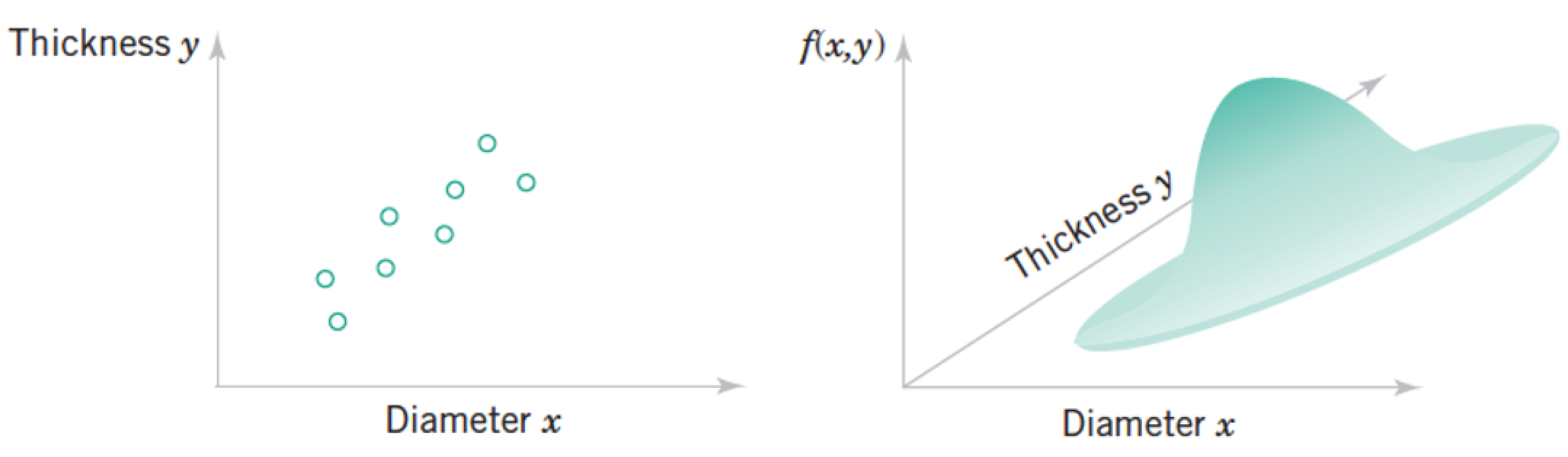
Each "sample" as a list of features, which we model as a vector of random variables, $$ \mathbf x = \begin{pmatrix} Diameter \\ Thickness \end{pmatrix} = \begin{pmatrix} x_1 \\ \vdots \\ x_n \\ \end{pmatrix} \rightarrow p(\mathbf x) = p(x_1, x_2) = p(\text{thickness, diameter}) $$

Each point in the distribution is simultanous probability of all the features taking the particular vector of numbers at the point.

Using Structure

Joint distribution: $p(\text{temperature anomaly}, \text{$CO_2$ concentration})$

Correlations are useful, whether due to causality or a common cause

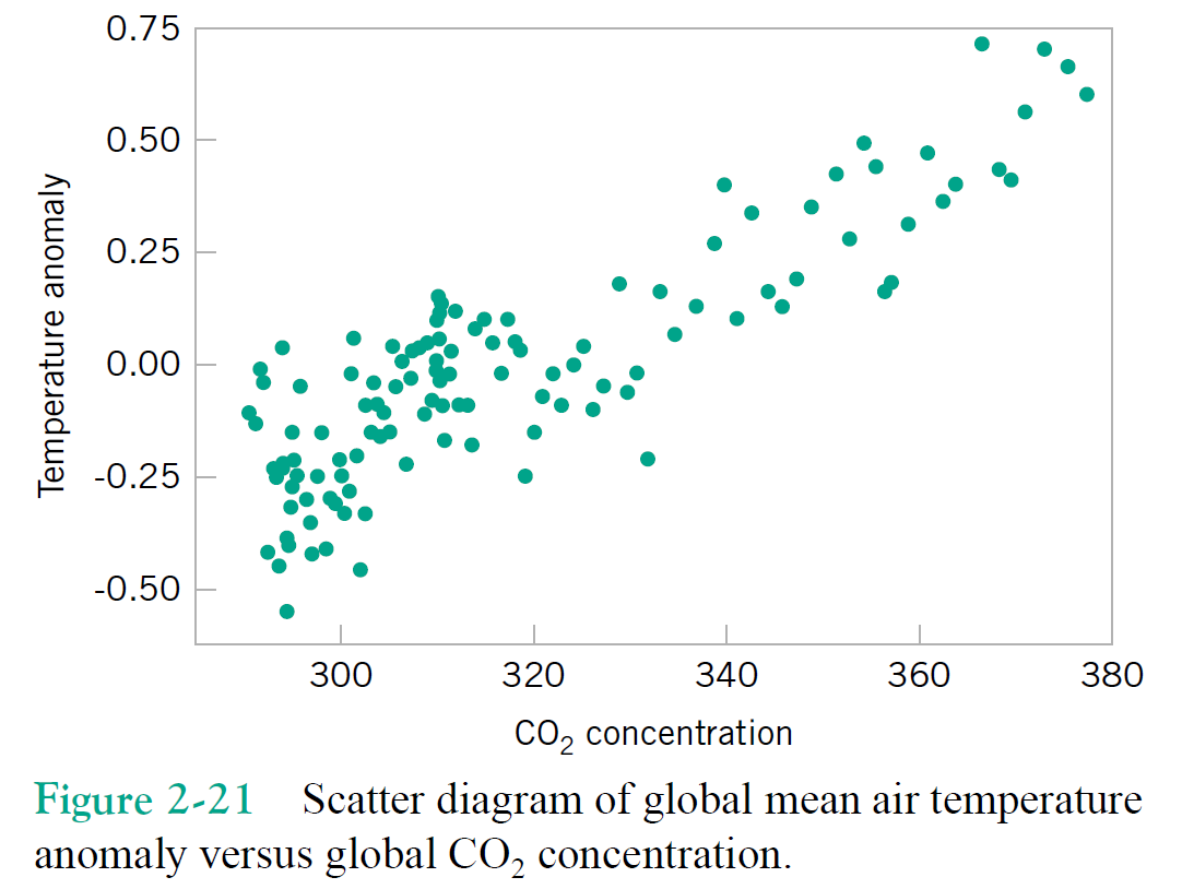
If I know the $CO_2$ concentration is over 400, what do I expect the temerature anomaly to be?

$$p(\text{temperature anomaly | concentration})$$

Fitting a model

Generally given a $CO_2$ concentration of $x_i$, what is the corresponding temperature anomaly, "$y(x_i)$" (approximately)

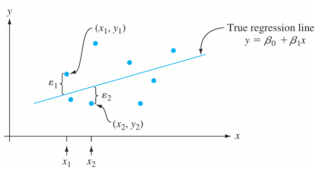
Choose to use a model of the form $y(x) = \beta_0 + \beta_1 x$, where $fitting$ refers to the choice of the best $\beta_0$ and $\beta_1$ -> choose slope and intercept

Two separate "functions" here: the probability distribution $p(x,y)$, and the regression model $\hat{y}(x_i) \approx y_i$

Devore, "Probability and Statistics for Engineering and the Sciences", Brooks. (2000).

The error terms $\varepsilon_i$ are assumed to be just uninteresting random values ~ noise

Example

print ("dosage = "+str(np.round(dosage,2)))
print ("blood concentration = "+str(np.round(conc_noisy,2)))

dosage = [   0.    166.67  333.33  500.    666.67  833.33 1000.  ]
blood concentration = [33.52 42.77 -9.23 12.1  36.8  69.32 59.61]

We have data for drug dosage and resulting blood concentration of drug.

We want a model to predict how much dosage to give to achieve a desired blood concentration.

1st order Polynomial Fit

poly_ex_1 = np.polyfit(dosage,conc_noisy,1)
show_polyfit_example_results(dosage, conc_true,conc_noisy,poly_ex_1,1)

true intercept: 10.0, est: 15.973; true slope: 0.05, est: 0.038

"true"means the numerical model used to generate the numbers here. Before adding random numbers to simulate noise.

Exercise 0: Literally do this in Python

dosage = np.array([0., 166.67, 333.33, 500., 666.67, 833.33, 1000.])
blood_concentration = np.array([35.07, 3.18, 26.43, 23.36, 47.93, 72.21, 62.78])

Estimate the relationship between dosage and blood_concentration by guessing slope/intercept

plt.plot(dosage, blood_concentration,'o-')
slope = 5 # a.k.a. beta_1, try and find better values than this...
intercept = 20  # a.k.a. beta_0, try and find better values than this...
plt.plot(dosage, slope*dosage+intercept) 
plt.xlabel('dosage (a.k.a. x)')
plt.ylabel('blood concentration (a.k.a. y)');

How well fit?

• How might we decide how accurate the fit is?

show_polyfit_example_results(dosage, conc_true,conc_noisy,poly_ex_1,1)

true intercept: 20, est: 15.973; true slope: 5, est: 0.038

Residual

import numpy as np
from matplotlib import pyplot as plt
x = np.linspace(0, 10, 100)
y = 2*x+3
s = 0.4

plt.plot(x, y, 'k-');
plt.plot([1, 1, 2, 3, 3, 4, 4, 5, 6, 7],[7, 3, 12, 5, 11, 15, 10, 15, 12, 19], 'yo', markersize=7);
plt.plot([1, 1], [7-s, 5], 'b-', [1, 1], [3+s, 5], 'b-', [2, 2], [12-s, 7], 'b-', [3, 3], [5+s, 9], 'b-', [3, 3], [11-s, 9], 'k-', [4,4], [15-s, 11], 'b-',          [4,4], [10+s, 11], 'b-', [5, 5], [15-s, 13], 'b-', [6, 6], [12+s+0.1, 15], 'b-', [7, 7], [19-s, 17], 'b-', linestyle='dashed');

C:\Users\micro\AppData\Local\Temp\ipykernel_34436\2661373173.py:9: UserWarning: linestyle is redundantly defined by the 'linestyle' keyword argument and the fmt string "b-" (-> linestyle='-'). The keyword argument will take precedence.
  plt.plot([1, 1], [7-s, 5], 'b-', [1, 1], [3+s, 5], 'b-', [2, 2], [12-s, 7], 'b-', [3, 3], [5+s, 9], 'b-', [3, 3], [11-s, 9], 'k-', [4,4], [15-s, 11], 'b-',          [4,4], [10+s, 11], 'b-', [5, 5], [15-s, 13], 'b-', [6, 6], [12+s+0.1, 15], 'b-', [7, 7], [19-s, 17], 'b-', linestyle='dashed');
C:\Users\micro\AppData\Local\Temp\ipykernel_34436\2661373173.py:9: UserWarning: linestyle is redundantly defined by the 'linestyle' keyword argument and the fmt string "k-" (-> linestyle='-'). The keyword argument will take precedence.
  plt.plot([1, 1], [7-s, 5], 'b-', [1, 1], [3+s, 5], 'b-', [2, 2], [12-s, 7], 'b-', [3, 3], [5+s, 9], 'b-', [3, 3], [11-s, 9], 'k-', [4,4], [15-s, 11], 'b-',          [4,4], [10+s, 11], 'b-', [5, 5], [15-s, 13], 'b-', [6, 6], [12+s+0.1, 15], 'b-', [7, 7], [19-s, 17], 'b-', linestyle='dashed');

How would you set this up mathematically?

Simple Linear Regression

Model assumption: $\mathbf y$ and $\mathbf x$ are linearly related

$$\mathbf y = \beta_0 + \beta_1 \mathbf x + \boldsymbol\varepsilon$$

$$\text{where } \mathbf y = \begin{bmatrix} y_1 \\y_2 \\ \vdots \\ y_m \end{bmatrix}, \;\; \mathbf x = \begin{bmatrix} x_1 \\x_2 \\ \vdots \\ x_m \end{bmatrix}, \;\; \boldsymbol\varepsilon = \begin{bmatrix} \varepsilon_1 \\ \varepsilon_2 \\ \vdots \\ \varepsilon_m \end{bmatrix}$$

How does this model apply to our example? What is $x_i$?

The Noise $\boldsymbol\varepsilon$

Basically the model is saying $\mathbf y \approx \beta_0 + \beta_1 \mathbf x$.

How approximate? Well the residual $\boldsymbol\varepsilon = \mathbf y - (\beta_0 + \beta_1 \mathbf x)$ is random --> so give it a statistical model

E.g., zero-mean, Gaussian. Educated guesses? Are they correct?

Answers:

• Law of large numbers makes things look Gaussian

• mean and variance can be measured from data -> Normality tests

• zero-mean can be enforced.

Residual on Data

print ("blood conc (measured) = "+str(np.round(conc_noisy,2)))
print ("blood conc (model) = "+str(np.round(np.polyval(poly_ex_1,dosage),2)))
print ("difference = "+str(np.round(conc_noisy - np.polyval(poly_ex_1,dosage),2)))

plt.scatter(dosage, conc_noisy , color='red')
plt.scatter(dosage, np.polyval(poly_ex_1,dosage) , color='black');
plt.plot(dosage, np.polyval(poly_ex_1,dosage) , color='black', linewidth="1");

blood conc (measured) = [33.52 42.77 -9.23 12.1  36.8  69.32 59.61]
blood conc (model) = [15.97 22.31 28.65 34.98 41.32 47.65 53.99]
difference = [ 17.54  20.46 -37.88 -22.88  -4.52  21.66   5.62]

Ordinary Least Squares - minimizes the residual

• Minimizes $\Vert \mathbf e \Vert_2^2 = \sum_{i=1}^n e_i^2$ where $\bf e = \beta_0 + \beta_1 \mathbf x - \mathbf y$, wrt $\beta_0$ and $\beta_1$

• In the simple linear regression case,

  $\hat{\beta}_1 = \frac{\sum_{i=1}^n (x_i - \bar{x})(y_i - \bar{y})}{\sum_{i=1}^n (x_i - \bar{x})^2}$, or

  $\hat{\beta}_1 = r_{xy} \frac{s_y}{s_x}$, where $r_{xy}$ is the correlation between $\mathbf x$ and $\mathbf y$, $s_x$ and $s_y$ are the standard deviations of $\mathbf x$ and $\mathbf y$

  $\hat{\beta}_0 = \bar{y} - \hat{\beta}_1 \bar{x}$

Exercise:

Perform this optimization for cases with just $\beta_0$ and just $\beta_1$.

1. Minimize $\sum_{i=1}^n e_i^2$ where $\bf e = \beta_0 - \mathbf y$ wrt $\beta_0$

2. Minimize $\sum_{i=1}^n e_i^2$ where $\bf e = \beta_1 \mathbf x - \mathbf y$ wrt $\beta_1$

Coefficient of Determination $R^2$

$$ R^2 = \frac{TSS-RSS}{TSS} $$

• TSS = Total sum of squares: $\sum_{i=1}^n (y_i - \bar{y})^2$ ~ variance (scaled)
• RSS = Residual sum of squares: $\sum_{i=1}^n e_i^2 = \sum_{i=1}^n (y_i - \hat{y}_i)^2$ ~ "noise" variance

The fraction of unexplained variance.

See Ch. 3, especially Eqs. 3.16-3.17 in "An Introduction to Statistical Learning". James, Witten, Hastie and Tibshirani, https://www-bcf.usc.edu/~gareth/ISL/

Exercise

Compute the residual for your estimate from Exercise 0

Apply it

Recall single-variable regression: find parameters ($\beta^*_0, \beta^*_1$) that minimize $residual = \sum_i e_i^2 = \Vert \mathbf e \Vert^2 = \Vert \mathbf y - f(\mathbf x;\beta_0, \beta_1) \Vert^2$

What is the (regular) algebra equation to predict global temperature $T$ using time $t$? $(t_1,T_1),(t_2,T_2),...,(t_m,T_m)$ $\rightarrow$?

$(t_1,s_1,T_1),(t_2,s_2,T_2),...,(t_m,s_m,T_m)$ $\rightarrow$?

What is the difference between minimizing norm of residual and variance of residual?

Better fit means better model... right?

show_polyfit_example_results(dosage, conc_true,conc_noisy,poly_ex_1,1)

true intercept: 20, est: 15.973; true slope: 5, est: 0.038

Brain teaser: Which fits the data better, the truth or our estimate? why?

GENERALIZATION

Machine Learning's goal is to find model which best fits new data best.

I.e., we want a predictor.

• Training set - the data we use for fit

• Test set - additional data we test on -> is the model still best?

Ironically, best model generally does not fit our training set best.

Caution

If you use the data at all to determine the model, you are cheating if you use it for final testing. Info leaks in, and overfitting occurs to a degree. Examples, using all data to:

• Standardize or subtracting mean
• Picking out best-looking features
• Choosing model and/or parameters
• Even choosing parameters from cross-validation

Ideal plan is separate training, validation, and test sets.

May have no choice if data is too limited however.

Cross-Validation

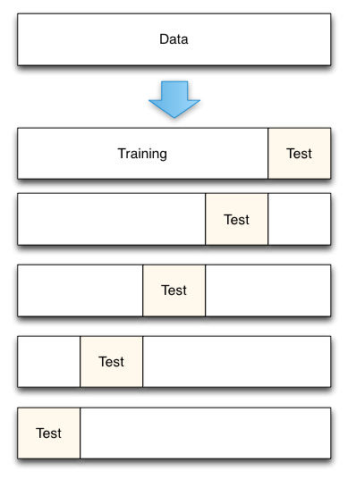
http://scikit-learn.org/stable/modules/classes.html

How does this apply to our typical data matrix?

PRO TIP: if standardizing, use mean & std of training set.

Multi-variable Regression

Recall Simple Linear Regression

Have data $\mathbf x$ and $\mathbf y$

1-D model: ${\mathbf y} = \beta_0 + \beta_1 \mathbf x + \boldsymbol\varepsilon$

• where $\mathbf y = \begin{bmatrix} y_1 \\y_2 \\ \vdots \\ y_m \end{bmatrix}$, $\mathbf x = \begin{bmatrix} x_1 \\x_2 \\ \vdots \\ x_m \end{bmatrix}$, $\boldsymbol\varepsilon = \begin{bmatrix} \varepsilon_1 \\ \varepsilon_2 \\ \vdots \\ \varepsilon_m \end{bmatrix}$

Remember what these terms are?

Multi-variable Model

New model: $\mathbf y = \beta_0 + \beta_1 \mathbf x_{(1)} + \beta_2 \mathbf x_{(2)} +...+ \beta_n \mathbf x_{(n)} + \boldsymbol\varepsilon$

• where $\mathbf y = \begin{bmatrix} y_1 \\y_2 \\ \vdots \\ y_n \end{bmatrix}$, $\mathbf x_{(i)} = \begin{bmatrix} x_{(i),1} \\x_{(i),2} \\ \vdots \\ x_{(i),m} \end{bmatrix}$, $\boldsymbol\varepsilon = \begin{bmatrix} \varepsilon_1 \\ \varepsilon_2 \\ \vdots \\ \varepsilon_n \end{bmatrix}$

E.g., predict temperature using: time of year, time of day, and lattitude, to get more accurate prediction.

Multi-variable Model, Matrix-style $x_{(j),i} \rightarrow X_{i,j}$

\begin{align} \mathbf y &= \beta_0 + \beta_1 \mathbf x_{(1)} + \beta_2 \mathbf x_{(2)} +...+ \beta_n \mathbf x_{(n)} + \boldsymbol\varepsilon \\ &= \beta_0 + \mathbf X \boldsymbol\beta + \boldsymbol\varepsilon \end{align}

• where $\mathbf y = \begin{bmatrix} y_1 \\y_2 \\ \vdots \\ y_n \end{bmatrix}$, $\boldsymbol\beta = \begin{bmatrix} \beta_1 \\ \beta_2 \\ \vdots \\ \beta_m \end{bmatrix}$, $\boldsymbol\varepsilon = \begin{bmatrix} \varepsilon_1 \\ \varepsilon_2 \\ \vdots \\ \varepsilon_n \end{bmatrix}$,

and $X_{i,j}$ is our well-known data matrix, features $\times$ samples.

Pesky Offset Term

Notice we've been adding a scalar to vectors $\beta_0 + \mathbf X \boldsymbol\beta + \boldsymbol\varepsilon$

1. This can be written more carefully using a vector of 1's.

\begin{align} \mathbf y &= \beta_0 \mathbf 1 + \beta_1 \mathbf x_{(1)} + \beta_2 \mathbf x_{(2)} +...+ \beta_n \mathbf x_{(n)} + \boldsymbol\varepsilon \\ &= \beta_0 \mathbf 1 + \mathbf X \boldsymbol\beta + \boldsymbol\varepsilon \end{align}

• How might we simplify this further (Hint: set $\mathbf x_{(0)} = \bf 1$)?

2. What if we standardize the data (or just removed the means)?

...."without loss of generality"

Exercise

What is the (regular) algebra equation to predict global temperature $T$ using time and $CO_2$ $s$?

$(t_1,s_1,T_1),(t_2,s_2,T_2),...,(t_m,s_m,T_m)$ $\rightarrow$?

Statistical model

Let $y_i = \beta_0 + \beta_1 X_{i,1} + ... + \beta_n X_{i,N} + \boldsymbol\varepsilon_i$ where $\varepsilon \sim N(0,\sigma^2)$

$X_{i,j} = x_{(i),j}$ are our observations, the $j$th observation for the $i$th variable.

Therefore each $y_i$ is also normally distributed with a mean value of $\beta_0 + \beta_1 X_{i,1} + ... + \beta_n X_{i,N}$ and a variance of $\sigma^2$

In other words: $$p(y_i|\beta_0, \beta_1, ..., \beta_N, X_{i,1},...,X_{i,N}) = \frac{1}{\sqrt{2\pi\sigma^2}} \exp{\left(\frac{-1}{2\sigma^2} \left(y_i - (\beta_0 + \beta_1 X_{i,1} + ... + \beta_n X_{i,N})\right)^2\right)}$$

Model for an entire dataset, $i=1...M$

Assumption: measurements are IID ~ independent and identically-distributed -> product of individual distributions

\begin{align} p(y_1, y_2, ..., y_M|\beta_0, \beta_1, ..., \beta_N, x_{1,1}, ..., x_{M,N}) &= p(\mathbf y |\boldsymbol\beta, \mathbf X) = \prod_i^M \frac{1}{\sqrt{2\pi\sigma^2}} \exp{\left(\frac{-1}{2\sigma^2} \left(y_i - (\beta_0 + \beta_1 X_{i,1} + ... + \beta_n X_{i,N})\right)^2\right)} \end{align}

\begin{align} p(\mathbf y |\boldsymbol\beta, \mathbf X) &= \prod_i^M \frac{1}{\sqrt{2\pi\sigma^2}} \exp{\left(\frac{-1}{2\sigma^2} \left(y_i - (\beta_0 + \beta_1 X_{i,1} + ... + \beta_n X_{i,N})\right)^2\right)} \\ &= \frac{1}{\sqrt{2\pi\sigma^2}^N} \exp{ \left( \sum_i^N\frac{-1}{2\sigma^2} \left(y_i - (\beta_0 + \beta_1 X_{i,1} + ... + \beta_n X_{i,N})\right)^2\right)} \\ &= \frac{1}{\sqrt{2\pi\sigma^2}^N} \exp{ \left(\frac{-1}{2\sigma^2} \Vert\mathbf y -\mathbf X \boldsymbol{\beta}\Vert_2^2 \right)} \\ &= \frac{1}{\sqrt{2\pi\sigma^2}^N} \exp{ \left(\frac{-1}{2} (\mathbf y -\mathbf X \boldsymbol{\beta})^T\boldsymbol\Sigma^{-1} (\mathbf y -\mathbf X \boldsymbol{\beta}) \right)} \\ \end{align}

$$\text{Where } \boldsymbol{\beta} = \begin{pmatrix}\beta_0\\ \beta_1\\ \vdots \\ \beta_N \end{pmatrix}, \;\; \mathbf X = \begin{pmatrix}1 & X_{1,1} & X_{1,2} & \dots & X_{1,n}\\ 1 & X_{1,2} & X_{2,2} & \dots & X_{2,n} \\ \vdots & \vdots & \vdots & & \vdots \\ 1 & X_{m,1} & X_{m,2} & \dots & X_{m,n} \end{pmatrix}, \;\; \boldsymbol\Sigma^{-1} = \frac{1}{\sigma^2} \mathbf I $$

Maximum Likelihood estimate

Maximum likelihood approach seeks the model which maximizes the probability of the measured data ${y_i}$ given the "inputs" ${X_{i,j}}$

This means find the $\boldsymbol\beta^*$ for which $p(\mathbf y| \boldsymbol\beta, \mathbf X)$ is largest for some data $(\mathbf y, \mathbf X)$ that you have

$$p(\mathbf y | \boldsymbol\beta, \mathbf X) = \frac{1}{\sqrt{2\pi\sigma^2}^N} \exp{ \left(\frac{-1}{2\sigma^2} \Vert\mathbf y -\mathbf X \boldsymbol{\beta}\Vert_2^2 \right)}$$

The Art of Optimization

$$\arg\max\limits_{\ \boldsymbol\beta}p(\mathbf y|\boldsymbol\beta, \mathbf X) = \arg\max\limits_{ \boldsymbol\beta} \left\{ \frac{1}{\sqrt{2\pi\sigma^2}^N} \exp{ \left(\frac{-1}{2\sigma^2} \Vert\mathbf y -\mathbf X \boldsymbol{\beta}\Vert_2^2 \right)} \right\} $$

$$= \arg\max\limits_{ \boldsymbol\beta} \ln \left\{ \frac{1}{\sqrt{2\pi\sigma^2}^N} \exp{ \left(\frac{-1}{2\sigma^2} \Vert\mathbf y -\mathbf X \boldsymbol{\beta}\Vert_2^2 \right)} \right\} $$

$$= \arg\max\limits_{ \boldsymbol\beta} \left[ \ln \left\{ \frac{1}{\sqrt{2\pi\sigma^2}^N} \right\} + \ln\left\{ \exp{ \left(\frac{-1}{2\sigma^2} \Vert\mathbf y -\mathbf X \boldsymbol{\beta}\Vert_2^2 \right)} \right\} \right] $$

$$= \arg\max\limits_{ \boldsymbol\beta} \left(\frac{-1}{2\sigma^2} \Vert\mathbf y -\mathbf X \boldsymbol{\beta}\Vert_2^2 \right) $$

$$ = \arg\min\limits_{ \boldsymbol\beta} \Vert\mathbf y -\mathbf X \boldsymbol{\beta}\Vert_2^2 $$

Optimization aside

A framework for describing problems for minimizing/maximizing functions Plus an "art" for finding easier alternative problems that have same minimizer.

\begin{align} \text{minimizer: } \mathbf z^* &= \arg\min\limits_{\mathbf z} g(\mathbf z) \\ \text{minimum: } g_{min} &= \min\limits_{\mathbf z} g(\mathbf z) = g(\mathbf z^*) \end{align}

\begin{align} \text{maximizer: } \mathbf z^* &= \arg\max\limits_{\mathbf z} g(\mathbf z) \\ \text{maximum: } g_{min} &= \max\limits_{\mathbf z} g(\mathbf z) = g(\mathbf z^*) \end{align}

What is "$g$" and $\mathbf z$ for our regression problem? for KNN? Naive Bayes?

Note 1: nuanced jargon here, minimizer is location of minimum, not minimum value itself.

Note 2: we aren't concerned with local vs. global minima/maxima here. But know they differ.

Linear Algebra view of Regression

The ML solution to the multiple linear regression problem with Gaussian error

$$ \boldsymbol\beta^*= \arg\min\limits_{ \boldsymbol\beta} \Vert\mathbf y -\mathbf X \boldsymbol{\beta}\Vert_2^2 $$

$$\text{where } \mathbf y = \begin{bmatrix} y_1 \\y_2 \\ \vdots \\ y_n \end{bmatrix},\;\; \boldsymbol{\beta} = \begin{pmatrix}\beta_0\\ \beta_1\\ \vdots \\ \beta_N \end{pmatrix}, \;\; \mathbf X = \begin{pmatrix}1 & X_{1,1} & X_{1,2} & \dots & X_{1,n}\\ 1 & X_{1,2} & X_{2,2} & \dots & X_{2,n} \\ \vdots & \vdots & \vdots & & \vdots \\ 1 & X_{m,1} & X_{m,2} & \dots & X_{m,n} \end{pmatrix}, \;\; \boldsymbol\varepsilon = \begin{bmatrix} \varepsilon_1 \\ \varepsilon_2 \\ \vdots \\ \varepsilon_n \end{bmatrix}$$

Is, in linear algebra terminology, this is the least-squares solution to the linear system:

$$ \mathbf y =\mathbf X \boldsymbol{\beta} $$

Linear systems

$$ \mathbf y =\mathbf X \boldsymbol{\beta} $$

CASE 1: $\mathbf X$ square, invertible (a.k.a. nonsingular). Can solve with inverse (generally never do this).

$$ \boldsymbol{\beta} = \mathbf X^{-1} \mathbf y $$

CASE 2: $\mathbf X$ "short and fat", more unknowns than equations, underdetermined. Solve with pseudoinverse.

$$ \boldsymbol{\beta} = \mathbf X^\dagger \mathbf y = \mathbf X^T \left(\mathbf X\mathbf X^T\right)^{-1} \mathbf y $$

CASE 3: $\mathbf X$ "tall and thin", more equations than unknowns, overdetermined. Solve with pseudoinverse.

$$ \boldsymbol{\beta} = \mathbf X^\dagger \mathbf y = \left(\mathbf X^T\mathbf X\right)^{-1} \mathbf X^T \mathbf y $$

Note that $\mathbf X^\dagger = \mathbf X^{-1}$ when the inverse exists. There are yet more nuances regarding how to handle small singular values and other numerical issues. Linear algebra libraries often have a robust pinv function in addition to other options like solve or a backslash operator "A\b"

Exercise: networks

Recall Gaussian Graphical model can be formed via regression relating nodes. Give the linear systems to be solved for a network consisting of three nodes, where we have a vector of data describing each node.

Solving Linear System with the SVD

Consider how to solve a system with invertible $\mathbf X$ using its SVD and knowledge of the factors' properties

Next consider how you might extend this to a singular matrix. (Hint: will end up equivalent to the pseudoinverse solution).

Regression Error Metric Recap

• Mean-squared Error (MSE), $L^2$-norm of residual $\mathbf e = \mathbf y - \mathbf X \boldsymbol\beta$

• Error variance, STD.

• Coefficient of determination $R^2$ ~ error variance as fraction of total variance

All essentially same info in linear algebra versus statistics.

Machine Learning in extremely-small nutshell

1. Pick a model, e.g., $\mathbf y = \beta_0 + \beta_1 \mathbf x + \boldsymbol\varepsilon = f(\mathbf x;\beta_0, \beta_1) + \boldsymbol\varepsilon$

2. "Fit" model to your data by using your favorite optimization technique to find parameters ($\beta^*_0, \beta^*_1$) that minimize $residual = \Vert \mathbf y - f(\mathbf x;\beta_0, \beta_1) \Vert$

Lab

Load Boston house prices dataset.

Formulate linear system and try using inverse and pseudoinverse to solve.

Compute prediction and residual from result(s) using test data.

Use scikit to predict Boston house prices using linear regression.

Which appear to be the most important features?

from sklearn.datasets import load_boston
boston = load_boston()
print(dir(boston))
print(boston.data.shape)
print(boston.feature_names)
print(boston.DESCR)

['DESCR', 'data', 'feature_names', 'filename', 'target']
(506, 13)
['CRIM' 'ZN' 'INDUS' 'CHAS' 'NOX' 'RM' 'AGE' 'DIS' 'RAD' 'TAX' 'PTRATIO'
 'B' 'LSTAT']
.. _boston_dataset:

Boston house prices dataset
---------------------------

**Data Set Characteristics:**  

    :Number of Instances: 506 

    :Number of Attributes: 13 numeric/categorical predictive. Median Value (attribute 14) is usually the target.

    :Attribute Information (in order):
        - CRIM     per capita crime rate by town
        - ZN       proportion of residential land zoned for lots over 25,000 sq.ft.
        - INDUS    proportion of non-retail business acres per town
        - CHAS     Charles River dummy variable (= 1 if tract bounds river; 0 otherwise)
        - NOX      nitric oxides concentration (parts per 10 million)
        - RM       average number of rooms per dwelling
        - AGE      proportion of owner-occupied units built prior to 1940
        - DIS      weighted distances to five Boston employment centres
        - RAD      index of accessibility to radial highways
        - TAX      full-value property-tax rate per $10,000
        - PTRATIO  pupil-teacher ratio by town
        - B        1000(Bk - 0.63)^2 where Bk is the proportion of blacks by town
        - LSTAT    % lower status of the population
        - MEDV     Median value of owner-occupied homes in $1000's

    :Missing Attribute Values: None

    :Creator: Harrison, D. and Rubinfeld, D.L.

This is a copy of UCI ML housing dataset.
https://archive.ics.uci.edu/ml/machine-learning-databases/housing/


This dataset was taken from the StatLib library which is maintained at Carnegie Mellon University.

The Boston house-price data of Harrison, D. and Rubinfeld, D.L. 'Hedonic
prices and the demand for clean air', J. Environ. Economics & Management,
vol.5, 81-102, 1978.   Used in Belsley, Kuh & Welsch, 'Regression diagnostics
...', Wiley, 1980.   N.B. Various transformations are used in the table on
pages 244-261 of the latter.

The Boston house-price data has been used in many machine learning papers that address regression
problems.   
     
.. topic:: References

   - Belsley, Kuh & Welsch, 'Regression diagnostics: Identifying Influential Data and Sources of Collinearity', Wiley, 1980. 244-261.
   - Quinlan,R. (1993). Combining Instance-Based and Model-Based Learning. In Proceedings on the Tenth International Conference of Machine Learning, 236-243, University of Massachusetts, Amherst. Morgan Kaufmann.

Maximum a Posteriori (MAP) Estimation

Again the system: $\mathbf y = \mathbf X \boldsymbol\beta + \boldsymbol\varepsilon$.

Now we seek to maximize the posterior distribution $p(\boldsymbol\beta | \mathbf y; \mathbf X)$ (statisticians also call this maximum likelihood).

The noise is Normally distributed with $\boldsymbol\varepsilon \sim N(\mathbf 0,\sigma_2^2 \mathbf I)$.

Assume the solution has a prior $\boldsymbol\beta \sim N(\mathbf 0,\sigma_1^2 \mathbf I)$

Use Bayes Law to solve for the Posterior distribution $p(\boldsymbol\beta | \mathbf y) = \dfrac{p(\mathbf y |\boldsymbol\beta) p(\boldsymbol\beta)}{p(\mathbf y)}$

Make a simpler optimization problem for finding the maximizer $\boldsymbol\beta^*$ for this. Hint: the denominator does not depend on $\boldsymbol\beta$.

Regression as Optimization

\begin{align} \text{Linear Regression: } \boldsymbol\beta_{lr}^* &= \arg\min\limits_{\boldsymbol\beta} \Vert \mathbf y - \mathbf X \boldsymbol\beta \Vert^2\\ \text{Ridge Regression: } \boldsymbol\beta_{rr}^* &= \arg\min\limits_{\boldsymbol\beta} \Vert \mathbf y - \mathbf X \boldsymbol\beta \Vert^2 + \lambda \Vert \boldsymbol\beta \Vert^2 \end{align}

Note these can be solved analytically with pseudoinverse or SVD techniques (which also provide some diffent kinds of variants).

Take home Messages

• A quadratic residual minimization (e.g. norm-squared or variance) implies a Gaussian noise assumption.

• A quadratic Penalty term implies a Gaussian prior assumption

• The regularization parameter relates the variances of the noise and prior. Which we have to guess at (i.e. fit).

Maximum a Posterior (MAP) Estimation II: "Laplace prior"

Again the system: $\mathbf y = \mathbf X \boldsymbol\beta + \boldsymbol\varepsilon$.

The noise is Normally distributed with $\boldsymbol\varepsilon \sim N(\mathbf 0,\sigma_2^2 \mathbf I)$.

Now the solution has a prior $\boldsymbol\beta \sim C \exp\big( \sum_i^n |\beta_i|\big)$. $C$ is a constant. This is sometimes called a Laplace distribution.

Use Bayes Law to solve for the Posterior distribution.

Make a simpler optimization problem for finding the maximizer $\boldsymbol\beta^*$ for this.

FYI: Full-on Bayesian Inference

While MAP estimation uses Bayes Law, it is not called Bayesian inference.

Maximum Likelihood and MAP estimates are examples of "point estimates".

A Bayesian Inference technique estimates the entire posterior distribution, meaning $\boldsymbol\mu$ and $\boldsymbol\Sigma$ in the prior example.

From this we can estimate many things, such as,

• the mean value of $\boldsymbol\beta$ $\rightarrow$ a (better?) point estimate versus maximum.
• the variance of $\boldsymbol\beta$ $\rightarrow$ confidence intervals.

Take home Messages (updated)

• A $\ell_2$ residual minimization (e.g. norm-squared or variance) implies a Gaussian noise assumption.

• A $\ell_2$ Penalty term implies a Gaussian prior assumption

• A $\ell_1$ Penalty term implies a Laplace prior assumption

• The regularization parameter relates the variances of the noise and prior. Which we have to guess at (i.e. fit).

Regression as Optimization (updated)

\begin{align} \text{Linear Regression: } \boldsymbol\beta_{lr}^* &= \arg\min\limits_{\boldsymbol\beta} \Vert \mathbf y - \mathbf X \boldsymbol\beta \Vert_2^2\\ \text{Ridge Regression: } \boldsymbol\beta_{rr}^* &= \arg\min\limits_{\boldsymbol\beta} \Vert \mathbf y - \mathbf X \boldsymbol\beta \Vert_2^2 + \lambda \Vert \boldsymbol\beta \Vert_2^2 \\ \text{"LASSO": } \boldsymbol\beta_{lasso}^* &= \arg\min\limits_{\boldsymbol\beta} \Vert \mathbf y - \mathbf X \boldsymbol\beta \Vert_2^2 + \lambda \Vert \boldsymbol\beta \Vert_1 \end{align}

Also Logistic version of everything for Classification.

Nonlinear regression

Fitting a line works in some cases, but other kinds of curves might work better elsewhere

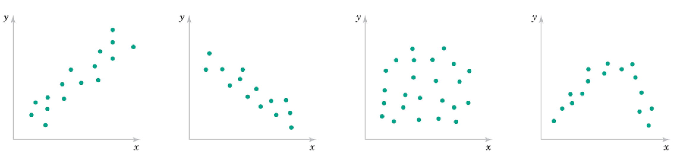
Suppose we know a relationship is quadratic

If we know the relationship is quadratic, we could just take the square root and make it linear.

Nonlinear regression (easy way) - Linear regression after nonlinear transformation

Old: \begin{align} \mathbf y = \beta_0 + \beta_1 \mathbf x_{(1)} + \beta_2 \mathbf x_{(2)} +...+ \beta_n \mathbf x_{(n)} + \varepsilon , \; \; \; \mathbf x_{(i)} = \begin{bmatrix} x_{(i),1} \\x_{(i),2} \\ \vdots \\ x_{(i),m} \end{bmatrix} \end{align}

New: \begin{align} \mathbf y = \beta_0 + \beta_1 \mathbf x'_{(1)} + \beta_2 \mathbf x'_{(2)} +...+ \beta_n \mathbf x'_{(n)} + \varepsilon, \;\;\; \mathbf x'_{(i)} = \begin{bmatrix} f_{(i)}(x_1) \\f_{(i)}(x_2) \\ \vdots \\ f_{(i)}(x_m) \end{bmatrix} \end{align}

...Feature Engineering, Kernel methods, ...

Polynomial regression - simple powers of data

New model: $\mathbf y = \beta_0 + \beta_1 \mathbf x'_{(1)} + \beta_2 \mathbf x'_{(2)} +...+ \beta_n \mathbf x'_{(n)} + \varepsilon$

$$\mathbf x'_{(i)} = \begin{bmatrix} f_{(i)}(x_1) \\f_{(i)}(x_2) \\ \vdots \\ f_{(i)}(x_m) \end{bmatrix} = \begin{bmatrix} x_{1}^i \\x_{2}^i \\ \vdots \\ x_{m}^i \end{bmatrix}$$

Exercise: write the model equations out for 3D case, i.e. $\bf x$ is just $x_1$, $x_2$, and $x_3$.

Polynomial regression

show_polyfit_ho_example_results(dosage,conc_noisy,(1,2,3,4,5,6));

order: 1, residual: 56.6204627002199
order: 2, residual: 43.28483436298878
order: 3, residual: 38.90189854595423
order: 4, residual: 21.166171682768383
order: 5, residual: 13.416800916508517
order: 6, residual: 1.8203750586044797e-11

Logistic regression

Logistic Regression: Motivation

NFL Example

• x axis is the number of touchdowns scored by team over a season
• y axis is whether they lost or won the game (0 or 1).

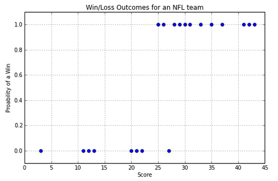
So, how do we predict whether we have a win or a loss if we are given a score? Note that we are going to be predicting values between 0 and 1. Close to 0 means we're sure it's in class 0, close to 1 means we're sure it's in class 1, and closer to 0.5 means we don't know.

Poorly fitting Linear Regression Model

Linear regression gets the general trend but it doesn't accurately represent the steplike behavior:

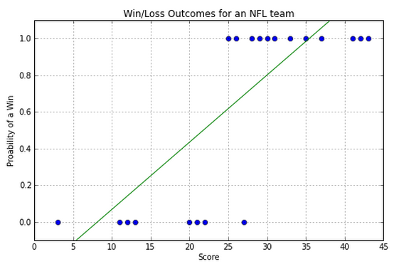
How would we use this model to estimate the class label (zero or one)?

Note mismatch between residual and "binarized" estimate.

So a line is not the best way to model this data. Luckily we know of a better curve.

Logistic Regression - fit sigmoid curve instead of line

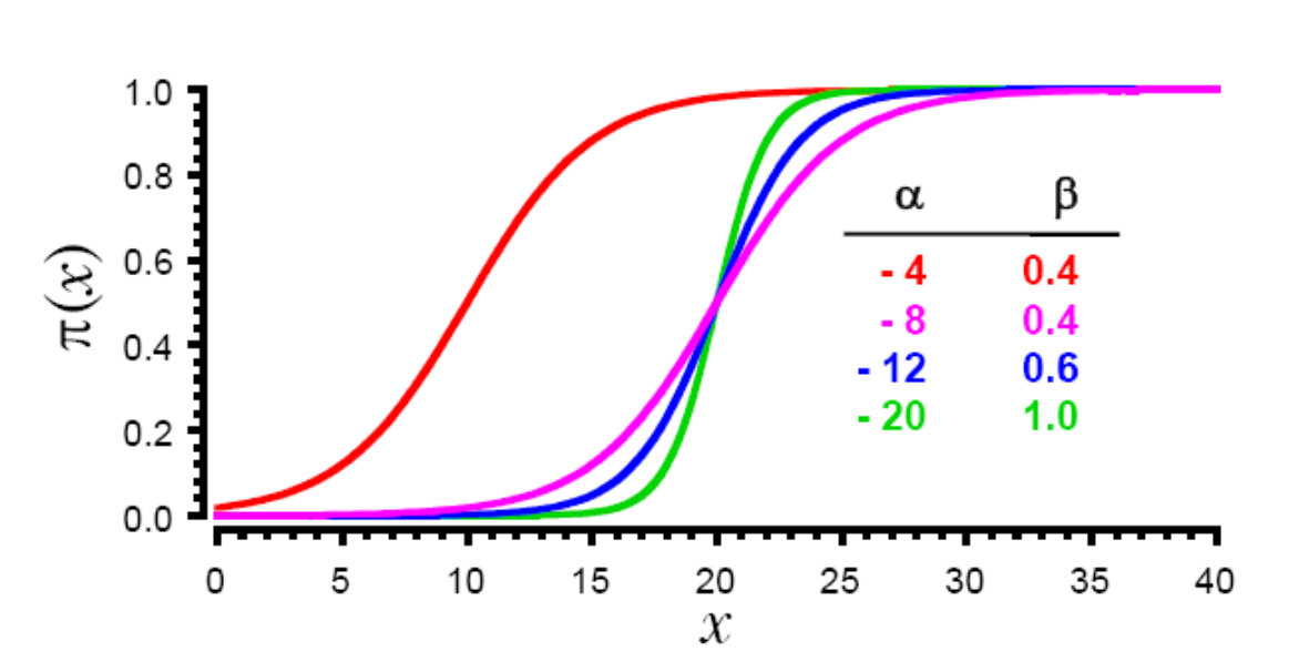
$$ "\pi(x)" = \frac{exp(\alpha+\beta x)}{1 + exp(\alpha+\beta x)} $$

Instead of choosing slope and intercept, choose parameters $\alpha$ and $\beta$ of sigmoid curve to fit the data.

Even easier to fit this one by eye in single variable case

Sigmoid, a.k.a. Standard Logistic Function

(Not the same as the standard deviation, just same symbol)

x = np.linspace(-10,10,100)

plt.figure(figsize=(8,2))
plt.plot(x,1/(1+np.exp(-1*x)), linewidth='1.7');
plt.plot(x,1/(1+np.exp(-2*x)), linewidth='1.7');
plt.plot(x,1/(1+np.exp(-1*(x+5))), linewidth='1.7');

plt.ylim(-0.001,1.01);
plt.legend((r'$\frac{1}{1+e^{-x}} = \sigma(x)$', r'$\frac{1}{1+e^{-2x}} = \sigma(2x)$', r'$\frac{1}{1+e^{-(x-5)}} = \sigma(x-5)$'), fontsize=14);
plt.grid();

Picture it: Classification versus Regression

• one-dimensional case

• two-dimensional case

What do binary labels look like in 1D versus 2D?

Lab

Use scikit-learn to perform classification using regression.

Try logistic, Ridge, and other regression methods.

Which are the most important features?

from sklearn.datasets import load_boston
boston = load_boston()
print(dir(boston))
print(boston.data.shape)
print(boston.feature_names)
print(boston.DESCR)

['DESCR', 'data', 'feature_names', 'filename', 'target']
(506, 13)
['CRIM' 'ZN' 'INDUS' 'CHAS' 'NOX' 'RM' 'AGE' 'DIS' 'RAD' 'TAX' 'PTRATIO'
 'B' 'LSTAT']
.. _boston_dataset:

Boston house prices dataset
---------------------------

**Data Set Characteristics:**  

    :Number of Instances: 506 

    :Number of Attributes: 13 numeric/categorical predictive. Median Value (attribute 14) is usually the target.

    :Attribute Information (in order):
        - CRIM     per capita crime rate by town
        - ZN       proportion of residential land zoned for lots over 25,000 sq.ft.
        - INDUS    proportion of non-retail business acres per town
        - CHAS     Charles River dummy variable (= 1 if tract bounds river; 0 otherwise)
        - NOX      nitric oxides concentration (parts per 10 million)
        - RM       average number of rooms per dwelling
        - AGE      proportion of owner-occupied units built prior to 1940
        - DIS      weighted distances to five Boston employment centres
        - RAD      index of accessibility to radial highways
        - TAX      full-value property-tax rate per $10,000
        - PTRATIO  pupil-teacher ratio by town
        - B        1000(Bk - 0.63)^2 where Bk is the proportion of blacks by town
        - LSTAT    % lower status of the population
        - MEDV     Median value of owner-occupied homes in $1000's

    :Missing Attribute Values: None

    :Creator: Harrison, D. and Rubinfeld, D.L.

This is a copy of UCI ML housing dataset.
https://archive.ics.uci.edu/ml/machine-learning-databases/housing/


This dataset was taken from the StatLib library which is maintained at Carnegie Mellon University.

The Boston house-price data of Harrison, D. and Rubinfeld, D.L. 'Hedonic
prices and the demand for clean air', J. Environ. Economics & Management,
vol.5, 81-102, 1978.   Used in Belsley, Kuh & Welsch, 'Regression diagnostics
...', Wiley, 1980.   N.B. Various transformations are used in the table on
pages 244-261 of the latter.

The Boston house-price data has been used in many machine learning papers that address regression
problems.   
     
.. topic:: References

   - Belsley, Kuh & Welsch, 'Regression diagnostics: Identifying Influential Data and Sources of Collinearity', Wiley, 1980. 244-261.
   - Quinlan,R. (1993). Combining Instance-Based and Model-Based Learning. In Proceedings on the Tenth International Conference of Machine Learning, 236-243, University of Massachusetts, Amherst. Morgan Kaufmann.

Quick Recap: Regression

$$\mathbf y = f(\mathbf x;\beta_0, \boldsymbol\beta) + \boldsymbol\varepsilon $$

Linear Regression: $f(\mathbf x;\beta_0, \boldsymbol\beta) = \beta_0 + \boldsymbol\beta x$, Logistic regression: $f(\mathbf x;\beta_0, \boldsymbol\beta) = \sigma(\beta_0 + \boldsymbol\beta x)$

Minimize $e^2 = \Vert \mathbf y - f(\mathbf x;\beta_0, \boldsymbol\beta) \Vert^2$ to find optimal $\boldsymbol\beta$ ~ LMS Loss

• Plan A. Guesstimate $\beta_0$, $\boldsymbol\beta$ by eye

• Plan B: analytically find minimizer using calculus

• Plan C: Use optimization - Newton method, LARS, gradient descent...

Regression for Classification

1. Simple Linear Regression, $f(\mathbf x;\beta_0, \boldsymbol\beta) = \beta_0 + \boldsymbol\beta^T \mathbf x$

Minimize $e^2 = \Vert \mathbf y - f(\mathbf x;\beta_0, \boldsymbol\beta) \Vert^2$ to find optimal $\boldsymbol\beta$ ~ LMS Loss, ak.a L2, Least Squares

2. Logistic Regression $f(\mathbf x;\beta_0, \boldsymbol\beta) = \sigma(\beta_0 + \boldsymbol\beta^T \mathbf x)$

$$\sigma(z) = \frac{1}{1+e^{-z}}$$

How might we fit this one?

one idea, do linear regression to fit then slap sigmoid on result

better way, do optimization with sigmoid in there (optimization harder now)

Statistical View (very quickly)

Bernoulli distribution:

\begin{align} \text{Prob}(Y=1) &= p, \;\; \text{Prob}(Y=0) = 1-p \end{align}

\begin{align} \text{Prob}(Y = y) &= p^y (1-p)^{(1-y)} \end{align}

Model the probability $p$ with sigmoid

\begin{align} \text{Prob}(Y = y) &= p^y (1-p)^y = \sigma(z)^y(1-\sigma(z))^{(1-y)} \end{align}

The likelihood of the data for this can be again formed by assuming independent measurements.

The log of the likelihood is called the Binary cross-entropy

Finding optimal parameters $\boldsymbol\beta$

Solving for the minimum by setting this derivative equal to zero doesn't work, but with enough time and computing resources you can minimize anything, especially if you can compute the gradient...

Gradient Descent

Went from too-trivial-to-cover in optimization classes, to the current state-of-the-art due to massive data sizes and parallel computing (scalability)

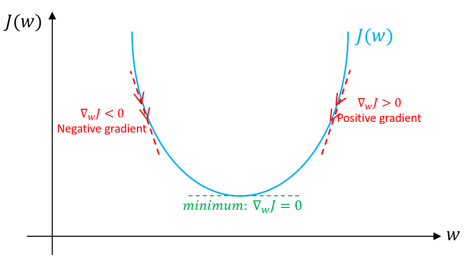
What do we use for the step size?

Multidimensional case: Matrix Calculus

https://en.wikipedia.org/wiki/Matrix_calculus

https://www.math.uwaterloo.ca/~hwolkowi/matrixcookbook.pdf

"The Matrix Calculus You Need For Deep Learning" https://arxiv.org/abs/1802.01528

Recap: Models

\begin{align} \text{General regression model: } y &= f(\boldsymbol\beta; \mathbf X)\\ \text{Linear regression: } y &= \beta_0 + \beta_1 x_1 + \beta_2 x_2 + ...\\ \text{Classification (Logistic regression): } y &= \sigma(\beta_0 + \beta_1 x_1 + \beta_2 x_2 + ...)\\ \text{Nonlinear regression model: } y &= \beta_0^{n} + \beta_1^{n} f_1(\mathbf x, \beta_1^{1,...,n-1}) + \beta_2^{n} f_2(\mathbf x, \mathbf \beta_2^{1,...,n-1}) + ...\\ \text{Nonlinear classification: } y &= \sigma\left(\beta_0^{n} + \beta_1^{n} f_1(\mathbf x, \beta_1^{1,...,n-1}) + \beta_2^{n} f_2(\mathbf x, \beta_2^{1,...,n-1}) + ...\right) \end{align}

Deep neural network

A series of "layers". Layer $i$ computes $y = "\sigma^{(i)}"(\beta_0 + \beta_1 x_1 + \beta_2 x_2 + ...)$

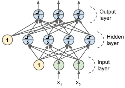
• "$\sigma^{(i)}$" are called the activation functions. Can be sigmoid, but ReLU very popular.

• $\beta$ the parameters are called weights

• Training = fitting the $\beta$ given a dataset