BDS 761: Data Science and Machine Learning I
Topic 4: Precision and Norms
This topic:
- Numerical precision (on modern desktop computers)
- Norms, distances, and basic stats
- k-means clustering
Readings:
- Intro to Applied Linear Algebra Ch. 3 & 4 https://web.stanford.edu/~boyd/vmls/
Numerical Precision
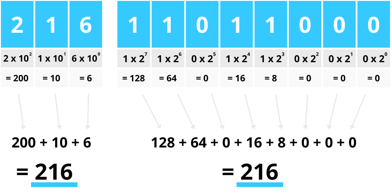
Binary numbers
https://mikkegoes.com/computer-science-binary-code-explained/
The basis for all modern computing.
What set of numbers can be represented with the above binary scheme and 8 bits?
What is the largest number possible with 8 bits? with 32 bits?
How many decimal digits do these amount to roughly?
bin(216) # gives binary representation of integer
'0b11011000'
import numpy as np

np.base_repr(216, base=2, padding=0)
'11011000'
Hexadecimal
Base-16 system. Effectively groups four binary digits into each hex digit.
for k in range(0,32):
    print(f'{k:4d}  {bin(k):>8s} {hex(k):>5s}.')
   0       0b0   0x0.
   1       0b1   0x1.
   2      0b10   0x2.
   3      0b11   0x3.
   4     0b100   0x4.
   5     0b101   0x5.
   6     0b110   0x6.
   7     0b111   0x7.
   8    0b1000   0x8.
   9    0b1001   0x9.
  10    0b1010   0xa.
  11    0b1011   0xb.
  12    0b1100   0xc.
  13    0b1101   0xd.
  14    0b1110   0xe.
  15    0b1111   0xf.
  16   0b10000  0x10.
  17   0b10001  0x11.
  18   0b10010  0x12.
  19   0b10011  0x13.
  20   0b10100  0x14.
  21   0b10101  0x15.
  22   0b10110  0x16.
  23   0b10111  0x17.
  24   0b11000  0x18.
  25   0b11001  0x19.
  26   0b11010  0x1a.
  27   0b11011  0x1b.
  28   0b11100  0x1c.
  29   0b11101  0x1d.
  30   0b11110  0x1e.
  31   0b11111  0x1f.
Floating point numbers
IEEE 754 standard for representing a real number with a 32-bit (or 64-bit) word.
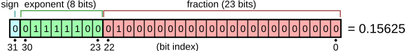
$$x = (-1)^{\text{sign}} \times \text{fraction} \times 2^\text{exponent}$$
Similar approach to achieve higher precision using 64-bit words
Note that two version of zero are possible, +0 and -0, depending on sign bit
$\pm$ Infinity = exponents all 1's, fraction all 0's
Not-a-number (NaN) = exponents all 1's, fraction not all 0's.
https://learn.microsoft.com/en-us/cpp/build/ieee-floating-point-representation?view=msvc-170
1./0.
---------------------------------------------------------------------------
ZeroDivisionError                         Traceback (most recent call last)
~\AppData\Local\Temp\ipykernel_26264\832528835.py in <module>
----> 1 1./0.

ZeroDivisionError: float division by zero
import numpy as np

1/np.array([0.]), -1./np.array([0.])
C:\Users\micro\AppData\Local\Temp\ipykernel_26264\3923875365.py:3: RuntimeWarning: divide by zero encountered in true_divide
  1/np.array([0.]), -1./np.array([0.])
(array([inf]), array([-inf]))
0.0/0.0
---------------------------------------------------------------------------
ZeroDivisionError                         Traceback (most recent call last)
~\AppData\Local\Temp\ipykernel_26264\1949058463.py in <module>
----> 1 0.0/0.0

ZeroDivisionError: float division by zero
0.0/np.array([0.0])
C:\Users\micro\AppData\Local\Temp\ipykernel_26264\844779733.py:1: RuntimeWarning: invalid value encountered in true_divide
  0.0/np.array([0.0])
array([nan])
0*np.nan
nan
np.inf*np.nan
nan
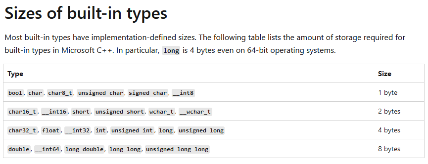
Commonly used number types
| Common names | bits |
|---|---|
| character (char) | 8 |
| integers (int) | 32 |
| unsigned integers (uint) | 32 |
| floating-pointing numbers (float, single) | 32,64 |
| double precision floating point numbers (double) | 64 |
| short integers (short) | 16 |
| long integers (long) | 32 |
| double long integers (longlong) | 64 |
| unsigned long integers (ulong) | 64 |
Note that number of bits used vary depending on hardware, compiler, ...
Precision (a.k.a. number of bits) is often added to the type name, e.g. float32.
Working with limited precision
Number of decimal digits from the number of binary exponent bits
- 32 bit floats have about 7 digits of precision
- 64 bit floats have about 16 digits precision
Must keep in mind that decimal numbers are always approximate.
1 + 1e-12
1.000000000001
1 + 1e-25
1.0
1 + 1e-25 == 1
True
1 + 1e-12 == 1
False
1e-25 + 1e-12
1.0000000000001e-12
A = np.random.randint(0, 10, size=(3, 3))
A_inv = np.linalg.inv(A)
print(A@A_inv) # matrix times its inverse should be identity
[[ 1.00000000e+00  0.00000000e+00 -2.22044605e-16]
 [-3.70074342e-18  1.00000000e+00  5.55111512e-17]
 [ 0.00000000e+00  0.00000000e+00  1.00000000e+00]]
Floating-Point Arithmetic
Floating point computations are not exact
$$ a+b \approx c$$Result will be nearest floating point number that can be represented with the binary system used.
hard zeros ~ special case when "0.0" really is all zeros (for fractional part) in binary
Logic, however, is still exact
0.1 + 0.1 + 0.1 == 0.3
False
0.1 + 0.1 + 0.1 + 0.1 + 0.1 + 0.1 + 0.1 + 0.1 + 0.1 + 0.1 == 1.0
False
round(0.1 + 0.1 + 0.1, 5) == round(0.3, 5) # round to 5 digits precision
True
import math

math.isclose(0.1 + 0.1 + 0.1, 0.3)
True
# but some calculations can still work

a=3
b=a/3
c=b*3
c==a
True
so what's the lesson here?
Overflow and Underflow
Overflow = not enough bits to represent number (number too big, positive or negative)
Underflow = not enough precision to represent number (number too small)
# Integer Overflow (int8)

import numpy as np

a = np.int8(120)
b = np.int8(10)
overflow_result = a + b
print("a =", a)
print("b =", b)
print("a + b =", overflow_result)  # Wraps around to a negative number
print("Expected (120 + 10) = 130, but stored as int8:", np.int8(130))
a = 120
b = 10
a + b = -126
Expected (120 + 10) = 130, but stored as int8: -126
C:\Users\micro\AppData\Local\Temp\ipykernel_11188\1159094512.py:7: RuntimeWarning: overflow encountered in byte_scalars
  overflow_result = a + b
# Integer Overflow (int16)

a16 = np.int16(32760)
b16 = np.int16(10)
print("a16 + b16 =", a16 + b16)  # Correct
print("int16 max =", np.iinfo(np.int16).max)

# Show overflow explicitly
overflow16 = np.int16(np.iinfo(np.int16).max + 1)
print("Overflow: int16(max + 1) =", overflow16)
a16 + b16 = -32766
int16 max = 32767
Overflow: int16(max + 1) = -32768
C:\Users\micro\AppData\Local\Temp\ipykernel_11188\934376104.py:5: RuntimeWarning: overflow encountered in short_scalars
  print("a16 + b16 =", a16 + b16)  # Correct
# Negative Integer "Overflow" (int8)

x = np.int8(-120)
y = np.int8(-10)
overflow_result = x + y
print("x =", x)
print("y =", y)
print("x + y =", overflow_result)  # Wraps around to a positive number
print("Expected (-120 - 10) = -130, but stored as int8:", np.int8(-130))
x = -120
y = -10
x + y = 126
Expected (-120 - 10) = -130, but stored as int8: 126
C:\Users\micro\AppData\Local\Temp\ipykernel_11188\1048983399.py:5: RuntimeWarning: overflow encountered in byte_scalars
  overflow_result = x + y
# Floating-Point Overflow
# This will overflow for float32 but not for float64

import numpy as np

a = np.float32(1e38)
b = np.float32(10)
overflow_result = a * b
print("a =", a)
print("b =", b)
print("a * b =", overflow_result)  # Will be inf
print("Is inf?", np.isinf(overflow_result))
a = 1e+38
b = 10.0
a * b = inf
Is inf? True
C:\Users\micro\AppData\Local\Temp\ipykernel_11188\591289397.py:8: RuntimeWarning: overflow encountered in float_scalars
  overflow_result = a * b
# Floating-Point Underflow

x = np.float32(1e-38)
y = np.float32(1e-10)
underflow_result = x * y
print("x =", x)
print("y =", y)
print("x * y =", underflow_result)  # Will be 0.0
print("Is zero?", underflow_result == 0.0)
x = 1e-38
y = 1e-10
x * y = 0.0
Is zero? True
# Float64 Example

a64 = np.float64(1e308)
b64 = np.float64(10)
print("a64 * b64 =", a64 * b64)  # Will overflow
--- Float64 Safe Example ---
a64 * b64 = inf
C:\Users\micro\AppData\Local\Temp\ipykernel_11188\1189525556.py:5: RuntimeWarning: overflow encountered in double_scalars
  print("a64 * b64 =", a64 * b64)  # Will overflow
x64 = np.float64(1e-308)
y64 = np.float64(1e-10)
print("x64 * y64 =", x64 * y64)  # Will underflow?
x64 * y64 = 1e-318
Preventing Overflow
Use larger number for result
import numpy as np

print("\n--- Preventing Overflow with Type Promotion ---")
# Start with int8
a = np.int8(120)
b = np.int8(10)

# Promote to int16 before addition
safe_result = np.int16(a) + np.int16(b)
print("a (int8) =", a)
print("b (int8) =", b)
print("a + b with int8 =", np.int8(a + b))  # Overflows
print("a + b with int16 =", safe_result)   # Correct result 130
--- Preventing Overflow with Type Promotion ---
a (int8) = 120
b (int8) = 10
a + b with int8 = -126
a + b with int16 = 130
C:\Users\micro\AppData\Local\Temp\ipykernel_11188\3938648987.py:12: RuntimeWarning: overflow encountered in byte_scalars
  print("a + b with int8 =", np.int8(a + b))  # Overflows
Precision Errors in Matrix Multiplication
Trade off precision for speed and memory use
import numpy as np
import time

# Matrix size
N = 1000  # Adjust based on system memory/performance

# Generate base float64 matrices from uniform [0, 255]
A64 = (np.random.rand(N, N) * 255).astype(np.float64)
B64 = (np.random.rand(N, N) * 255).astype(np.float64)

print("\n--- float64 ---")
size_bytes = A64.nbytes + B64.nbytes
print(f"Matrix size: {size_bytes / 1e6:.2f} MB")
start_time = time.time()
C64 = A64 @ B64
end_time = time.time()
print(f"Time taken: {end_time - start_time:.4f} seconds")

print("\n--- float32 ---")
A32 = A64.astype(np.float32)
B32 = B64.astype(np.float32)
size_bytes = A32.nbytes + B32.nbytes
print(f"Matrix size: {size_bytes / 1e6:.2f} MB")
start_time = time.time()
C32 = A32 @ B32
end_time = time.time()
print(f"Time taken: {end_time - start_time:.4f} seconds")

print("\n--- float16 ---")
A16 = A64.astype(np.float16)
B16 = B64.astype(np.float16)
size_bytes = A16.nbytes + B16.nbytes
print(f"Matrix size: {size_bytes / 1e6:.2f} MB")
start_time = time.time()
C16 = A16 @ B16
end_time = time.time()
print(f"Time taken: {end_time - start_time:.4f} seconds")

print("\n--- int32 ---")
Aint32 = A64.astype(np.int32)
Bint32 = B64.astype(np.int32)
size_bytes = Aint32.nbytes + Bint32.nbytes
print(f"Matrix size: {size_bytes / 1e6:.2f} MB")
start_time = time.time()
Cint32 = Aint32 @ Bint32
end_time = time.time()
print(f"Time taken: {end_time - start_time:.4f} seconds")

print("\n--- int64 ---")
Aint64 = A64.astype(np.int64)
Bint64 = B64.astype(np.int64)
size_bytes = Aint64.nbytes + Bint64.nbytes
print(f"Matrix size: {size_bytes / 1e6:.2f} MB")
start_time = time.time()
Cint64 = Aint64 @ Bint64
end_time = time.time()
print(f"Time taken: {end_time - start_time:.4f} seconds")

# Upsample results to float64 for fair comparison
C16_up = C16.astype(np.float64)
C32_up = C32.astype(np.float64)
Cint32_up = Cint32.astype(np.float64)
Cint64_up = Cint64.astype(np.float64)

# Compute maximum absolute differences
print("\n--- Maximum Absolute Differences ---")
print(f"max|C64 - C32| = {np.max(np.abs(C64 - C32_up)):.6e}")
print(f"max|C64 - C16| = {np.max(np.abs(C64 - C16_up)):.6e}")
print(f"max|C32 - C16| = {np.max(np.abs(C32_up - C16_up)):.6e}")
print(f"max|C64 - int32| = {np.max(np.abs(C64 - Cint32_up)):.6e}")
print(f"max|C64 - int64| = {np.max(np.abs(C64 - Cint64_up)):.6e}")
--- float64 ---
Matrix size: 16.00 MB
Time taken: 0.0224 seconds

--- float32 ---
Matrix size: 8.00 MB
Time taken: 0.0077 seconds

--- float16 ---
Matrix size: 4.00 MB
C:\Users\keith\AppData\Local\Temp\ipykernel_12860\449388697.py:35: RuntimeWarning: overflow encountered in matmul
  C16 = A16 @ B16
Time taken: 7.8111 seconds

--- int32 ---
Matrix size: 8.00 MB
Time taken: 2.1030 seconds

--- int64 ---
Matrix size: 16.00 MB
Time taken: 2.6975 seconds

--- Maximum Absolute Differences ---
max|C64 - C32| = 7.997219e+00
max|C64 - C16| = inf
max|C32 - C16| = inf
max|C64 - int32| = 1.394282e+05
max|C64 - int64| = 1.394282e+05
import numpy as np
import time

# Matrix size
N = 1000  # Adjust based on system memory/performance

# Generate base float64 matrices from uniform [0, 255]
A64 = (np.random.rand(N, N) * 255).astype(np.float64)
B64 = (np.random.rand(N, N) * 255).astype(np.float64)

print("\n--- float64 ---")
size_bytes = A64.nbytes + B64.nbytes
print(f"Matrix size: {size_bytes / 1e6:.2f} MB")
start_time = time.time()
C64 = A64 @ B64
end_time = time.time()
print(f"Time taken: {end_time - start_time:.4f} seconds")

print("\n--- float32 ---")
A32 = A64.astype(np.float32)
B32 = B64.astype(np.float32)
size_bytes = A32.nbytes + B32.nbytes
print(f"Matrix size: {size_bytes / 1e6:.2f} MB")
start_time = time.time()
C32 = A32 @ B32
end_time = time.time()
print(f"Time taken: {end_time - start_time:.4f} seconds")

print("\n--- float16 ---")
A16 = A64.astype(np.float16)
B16 = B64.astype(np.float16)
size_bytes = A16.nbytes + B16.nbytes
print(f"Matrix size: {size_bytes / 1e6:.2f} MB")
start_time = time.time()
C16 = A16 @ B16
end_time = time.time()
print(f"Time taken: {end_time - start_time:.4f} seconds")

print("\n--- int32 ---")
Aint32 = A64.astype(np.int32)
Bint32 = B64.astype(np.int32)
size_bytes = Aint32.nbytes + Bint32.nbytes
print(f"Matrix size: {size_bytes / 1e6:.2f} MB")
start_time = time.time()
Cint32 = Aint32 @ Bint32
end_time = time.time()
print(f"Time taken: {end_time - start_time:.4f} seconds")

print("\n--- int64 ---")
Aint64 = A64.astype(np.int64)
Bint64 = B64.astype(np.int64)
size_bytes = Aint64.nbytes + Bint64.nbytes
print(f"Matrix size: {size_bytes / 1e6:.2f} MB")
start_time = time.time()
Cint64 = Aint64 @ Bint64
end_time = time.time()
print(f"Time taken: {end_time - start_time:.4f} seconds")

# Upsample results to float64 for fair comparison
C16_up = C16.astype(np.float64)
C32_up = C32.astype(np.float64)
Cint32_up = Cint32.astype(np.float64)
Cint64_up = Cint64.astype(np.float64)

# Compute maximum absolute differences
print("\n--- Maximum Absolute Differences ---")
print(f"max|C64 - C32| = {np.max(np.abs(C64 - C32_up)):.6e}")
print(f"max|C64 - C16| = {np.max(np.abs(C64 - C16_up)):.6e}")
print(f"max|C32 - C16| = {np.max(np.abs(C32_up - C16_up)):.6e}")
print(f"max|C64 - int32| = {np.max(np.abs(C64 - Cint32_up)):.6e}")
print(f"max|C64 - int64| = {np.max(np.abs(C64 - Cint64_up)):.6e}")
--- float64 ---
Matrix size: 16.00 MB
Time taken: 0.1867 seconds

--- float32 ---
Matrix size: 8.00 MB
Time taken: 0.0340 seconds

--- float16 ---
Matrix size: 4.00 MB
C:\Users\micro\AppData\Local\Temp\ipykernel_11188\449388697.py:35: RuntimeWarning: overflow encountered in matmul
  C16 = A16 @ B16
Time taken: 6.0759 seconds

--- int32 ---
Matrix size: 8.00 MB
Time taken: 2.8536 seconds

--- int64 ---
Matrix size: 16.00 MB
Time taken: 3.8560 seconds

--- Maximum Absolute Differences ---
max|C64 - C32| = 1.330282e+01
max|C64 - C16| = inf
max|C32 - C16| = inf
max|C64 - int32| = 1.374838e+05
max|C64 - int64| = 1.374838e+05
Norms & Distances
Metric
Basically, boil multiple numbers (vectors, matrices, time series,...) or entire functions down to a single number
Examples
- GDP of economy
- BMI (body-mass index)
- A statistic (mean, variance, ...)
- Vector norms...
Always can be critized as discarding important info, but need to use something
Euclidean Norm
$$ \|x\| = \sqrt{x_1^2+x_2^2+\dotsb+x_n^2} $$"Length" of a vector (as opposed to length of the data structure, i.e. number of dimensions)
Also known as $\|x\|_2$, the "two-norm"
Example
$$\left\Vert \begin{pmatrix}2 \\ -1\\2 \end{pmatrix}\right\Vert = ?$$Also use a built-in function to do this
Exercise: give Euclidean norm using dot products
Root-mean-square value (RMS)
$$ rms(x) = \sqrt{\frac{x_1^2+x_2^2+\dotsb+x_n^2}{n}} = \frac{1}{\sqrt{n}}\|x\| $$root(mean(square(x)))
Exercise: give Euclidean norm of sum of vectors $x+y$ in terms of dot products
(use result of previous exercise and work only with vectors)
$$||x+y||_2 = \text{dot}(?,?) + \text{dot}(?,?) + ???$$$$ \sqrt{(x_1+y_1)(x_1+y_1) + (x_2+y_2)(x_2+y_2) + ... } = $$Chebychev Inequality
If $x$ is a length-$n$ vector with $k$ entries satisfying $|x_i|\ge a$ for some constant $a>0$, then
$$\frac{k}{n} \le \left( \frac{rms(x)}{a}\right)^2$$Basically tells how much elements can deviate from the rms
Derive by noting that $\Vert x\Vert^2 \ge ka^2$
Motivation for other types of norms
Consider the list of data for different "dimensions", for one person, product, etc.
Does it make sense to compute Euclidean distance to tell us how "big" the vector is?
Norms
A norm is a vector "length". Often denoted generally as $\Vert \mathbf x \Vert$.
Properties
- Non-negativity: $\Vert \mathbf x \Vert \geq 0$
- Zero upon equality: $\Vert \mathbf x \Vert = 0 \iff \mathbf x = \mathbf 0$
- Absolute scalability: $\Vert \alpha \mathbf x \Vert = |\alpha| \Vert \mathbf x \Vert$ for scalar $\alpha$
- Triangle Inequality: $\Vert \mathbf x + \mathbf z\Vert \leq \Vert \mathbf x\Vert + \Vert \mathbf z\Vert$
$p$-Norms
For any $n$-dimensional real or complex vector. i.e. $x \in \mathbb{R}^n \text{ or } \mathbb{C}^n$
$$ \|x\|_p = \left(|x_1|^p+|x_2|^p+\dotsb+|x_n|^p\right)^{\frac{1}{p}} $$$$ \|x\|_p = \begin{pmatrix}\sum_{i=1}^n{|x_i|^p} \end{pmatrix}^{\frac{1}{p}} $$Consider the norms we have looked at. What is $p$?
Famous "norms"
- $\ell_2$ norm
- $\ell_1$ norm
- $\ell_\infty$ norm
- $\ell_p$ norm
- "$\ell_0$" norm
Note we often lazily write these as e.g. "L2" norm
Exercise: Wite out the $p$-norms for a vector $x$ for $p$ = 1,2,0,$\infty$... $ \|x\|_p = \begin{pmatrix}\sum_{i=1}^n{|x_i|^p} \end{pmatrix}^{\frac{1}{p}} $
Exercise: test the conditions for each
import numpy as np

v = [1,3,1,4]

for p in range(1,10):
    print(p,np.power(sum(np.power(np.abs(np.array(v)),p)),1/p))
1 9.0
2 5.196152422706632
3 4.530654896083492
4 4.290915128445443
5 4.175344598847825
6 4.110988070009078
7 4.0723049678331895
8 4.048006070825583
9 4.032310478684122
Exercise
What are the norms of $\vec{a} = \begin{bmatrix}1\\3\\1\\-4\end{bmatrix}$ and $\vec{b} = \begin{bmatrix}2\\0\\1\\-2\end{bmatrix}$?
"Norm balls"
The Set $\{x | \Vert x \Vert_p \le 1 \}$, $ \|x\|_p = \begin{pmatrix}\sum_{i=1}^n{|x_i|^p} \end{pmatrix}^{\frac{1}{p}} $
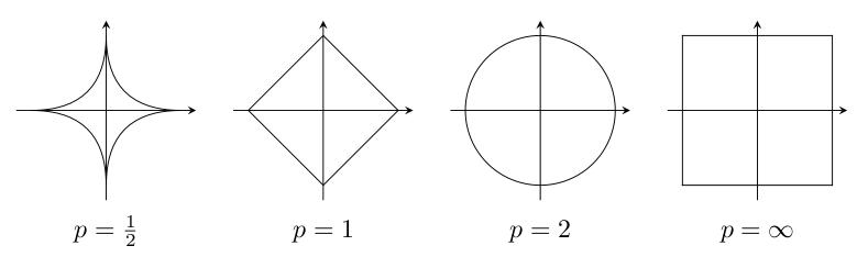
Note how $\Vert x \Vert_a \le \Vert x \Vert_b$ if $a\ge b$
Norms, Inner products, and angles
Inner product = length squared
$$v \cdot v = v^T v = \| v \|_2^2 = \| v \|_2\| v \|_2$$Angle $\theta$ between two vectors
$$v \cdot w = v^T w = \| v \|_2\| w \|_2 \cos\theta$$Cauchy-Schwartz Inequality $v^T w \le \| v \|\| w \|$
Triangle Inequality
$$\| v + w \| \le \| v \|+\| w \|$$Derive by noting that $\| v + w \|^2 = \|v\|^2 + v^Tw + \|w\|^2$ then use Cauchy-Schwartz and complete square
$S$-norm
For any symmetric positive definite matrix $S$
$$\| v \|_S^2 = v^T S v$$$S$ inner product
$$<v,w>_S = v^T S w$$Minkowski metric
Proposed by Lorentz for 4-dimensional spacetime, $v = (x,y,z,t)^T$, $c$ is speed of light
$$\| v\|^2_M = x^2+y^2+z^2-ct^2$$Is it a true norm?
II. Distances
Euclidean distance between two vectors $a$ and $b$ in $\mathbb{R}^{n}$:
$$d(\mathbf a,\mathbf b) = \sqrt{\sum_{i=1}^{n}(b_i-a_i)^2} = \Vert \mathbf b - \mathbf a \Vert_2$$Again this may not make sense for various vectors. Many alternatives...
Norm versus Distance
What is the relationship?
Distance properties
A distance metic $d(\mathbf x,\mathbf y)$ must satisfy four particular conditions to be considered a metric:
- Non-negativity: $d(\mathbf x,\mathbf y) \geq 0$
- Zero upon equality: $d(\mathbf x,\mathbf y) = 0 \iff \mathbf x = \mathbf y$
- Commutativity of arguments: $d(\mathbf x,\mathbf y) = d(\mathbf y,\mathbf x)$
- Triangle Inequality: $d(\mathbf x,\mathbf z) \leq d(\mathbf x,\mathbf y) + d(\mathbf y,\mathbf z)$
Exercise
Write the Euclidean distance between two points entirely in terms of dot products.
What does this tell you about using dot products to compare vector similarity?
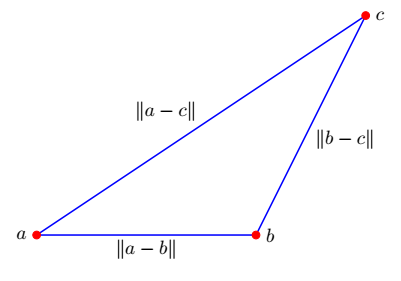
Triangle Inequality
$\Vert \mathbf x + \mathbf z\Vert \leq \Vert \mathbf x\Vert + \Vert \mathbf z\Vert$
$d(\mathbf a,\mathbf c) \leq d(\mathbf a,\mathbf b) + d(\mathbf b,\mathbf c)$
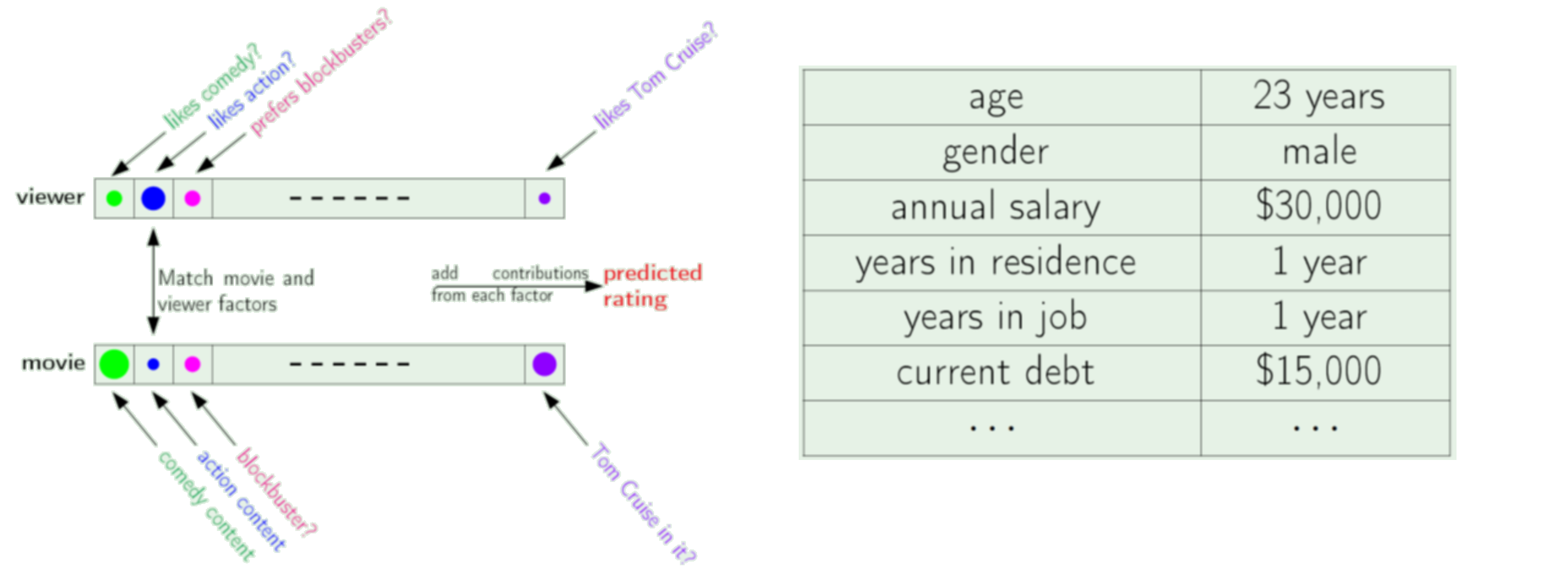
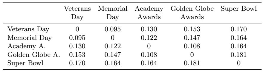
Application: feature distances
Recommender syatem based on most similar customers to movie properties
Question: what are the units of the distance here?
Application: rms prediction error
Time series prediction (stocks or temperature) compared to truth in retrospect
Manhattan or "Taxicab" Distance, also "Rectilinear distance"
Measures the relationships between points at right angles, meaning that we sum the absolute value of the difference in vector coordinates.
This metric is sensitive to rotation.
$$d_{M}(a,b) = \sum_{i=1}^{n}|b_i-a_i|$$Exercise
Does it fulfill the 4 conditions?
- Non-negativity: $d(\mathbf x,\mathbf y) \geq 0$
- Zero upon equality: $d(\mathbf x,\mathbf y) = 0 \iff \mathbf x = \mathbf y$
- Commutativity of arguments: $d(\mathbf x,\mathbf y) = d(\mathbf y,\mathbf x)$
- Triangle Inequality: $d(\mathbf x,\mathbf z) \leq d(\mathbf x,\mathbf y) + d(\mathbf y,\mathbf z)$
Chebyschev Distance
The Chebyschev distance or sometimes the $L^{\infty}$ metric, between two vectors is simply the the greatest of their differences along any coordinate dimension:
$$d_{\infty}(\mathbf a,\mathbf b) = \max_{i}{|(b_i-a_i)|}$$...consider
- Non-negativity: $d(\mathbf x,\mathbf y) \geq 0$
- Zero upon equality: $d(\mathbf x,\mathbf y) = 0 \iff \mathbf x = \mathbf y$
- Commutativity of arguments: $d(\mathbf x,\mathbf y) = d(\mathbf y,\mathbf x)$
- Triangle Inequality: $d(\mathbf x,\mathbf z) \leq d(\mathbf x,\mathbf y) + d(\mathbf y,\mathbf z)$
Cosine Distance
High school geometry: $\mathbf a \cdot \mathbf b = \|\mathbf a\|_2\|\mathbf b\|_2 \cos\theta$
Only depends on angle between the vectors
$$d_{\cos}(\mathbf a,\mathbf b) = 1-\frac{\mathbf a \cdot \mathbf b}{\|\mathbf a\|\|\mathbf b\|} = 1 - \cos\theta$$...consider (extra carefully)
- Non-negativity: $d(\mathbf x,\mathbf y) \geq 0$
- Zero upon equality: $d(\mathbf x,\mathbf y) = 0 \iff \mathbf x = \mathbf y$
- Commutativity of arguments: $d(\mathbf x,\mathbf y) = d(\mathbf y,\mathbf x)$
- Triangle Inequality: $d(\mathbf x,\mathbf z) \leq d(\mathbf x,\mathbf y) + d(\mathbf y,\mathbf z)$
Exercise
Implement the metrics manually and compute distances between:
$ \begin{bmatrix} 1 \\ 2 \\ 3 \\ 4 \end{bmatrix}$ and $ \begin{bmatrix} 5 \\ 6 \\ 7 \\ 8 \end{bmatrix}$
IV. Statistics with Python
Random sampling
- rand() - uniform random numbers in [0,1]
- randn() - standard normal random numbers (zero mean, unit variance)
from numpy import random

printcols(dir(random))
BitGenerator          __package__           default_rng           noncentral_chisquare  set_state
Generator             __path__              dirichlet             noncentral_f          shuffle
MT19937               __spec__              exponential           normal                standard_cauchy
PCG64                 _bounded_integers     f                     pareto                standard_exponential
PCG64DXSM             _common               gamma                 permutation           standard_gamma
Philox                _generator            geometric             poisson               standard_normal
RandomState           _mt19937              get_state             power                 standard_t
SFC64                 _pcg64                gumbel                rand                  test
SeedSequence          _philox               hypergeometric        randint               triangular
__RandomState_ctor    _pickle               laplace               randn                 uniform
__all__               _sfc64                logistic              random                vonmises
__builtins__          beta                  lognormal             random_integers       wald
__cached__            binomial              logseries             random_sample         weibull
__doc__               bit_generator         mtrand                ranf                  zipf
__file__              bytes                 multinomial           rayleigh
__loader__            chisquare             multivariate_normal   sample
__name__              choice                negative_binomial     seed
The Normal Distribution
- Also known as Gaussian distribution
import numpy as np
from matplotlib import pyplot as plt

def univariate_normal(x, mean, var):
    return ((1. / np.sqrt(2 * np.pi * var)) * np.exp(-(x - mean)**2 / (2 * var)))

x = np.linspace(-5,5,1000)
plt.plot(x,univariate_normal(x,1,2));
plt.show()

Exercise
Generate normal random samples with mean of 1 and variance of 1
Plot histogram versus the theoretical distribution
Try different numbers of samples
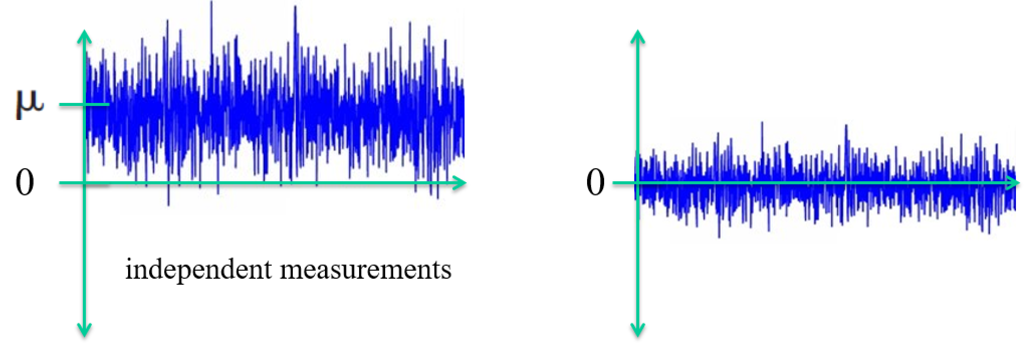
Statistics
Consider the relation between norms and simple statistical quantities
\begin{align} \text{Population mean} &= \mu = \frac{\sum_{i=1}^N x_i}{N} \\ \text{Sample mean} &= \bar{x} = \frac{\sum_{i=1}^n x_i}{n} \\ \text{Population variance} &= \sigma^2 = \frac{\sum_{i=1}^N (x_i - \mu)^2}{N} \\ \text{Sample variance} &= s^2 = \frac{\sum_{i=1}^n (x_i - \bar{x})^2}{n - 1} = \frac{\sum_{i=1}^n x_i^2 - \frac{1}{n}(\sum_{i=1}^n x_i)^2}{n - 1} \\ \text{Standard deviation} &= \sqrt{\text{Variance}} \end{align}Exercise
Load a dataset from sklearn and compute mean and variance of a column
Standardize the column
Now compute mean and variance of the result
The Standard Normal Distribution $Z$
- If $X$ is a normal r.v. with $E(X) = \mu$ and $V(X) = \sigma^2$
- $Z$ is a normal r.v. with $E(X) = 0$ and $V(X) = 1$
Standardizing data has two tasks
$$ Z = \frac{X-\mu}{\sigma} $$- Remove the mean
- scale by the standard deviation
Lab: Standardizing data
Standardize the columns of the Iris dataset using linear algebra.
Test it worked by computing the mean and norm of each column.
Multivariate Gaussian (for $n$ dimensions)
$$ f(\mathbf x) = \frac{1}{ \sqrt{2 \pi^n |\boldsymbol\Sigma|}} \exp \left(- \frac{1}{2} (\mathbf x - \boldsymbol \mu)^T \boldsymbol\Sigma^{-1} (\mathbf x - \boldsymbol \mu) \right) \text{, for } \mathbf x \in R^n $$- Mean vector as centroid of distribution
- Covariance matrix describes spread - correlations between variables $\Sigma_{ij} = S_{\mathbf x_i \mathbf x_j}$
def multivariate_normal(x, n, mean, cov):
    return (1./(np.sqrt((2*np.pi)**n * np.linalg.det(cov))) * np.exp(-1/2*(x - mean).T@np.linalg.inv(cov)@(x - mean)))


mean = np.array([35,70])
cov = 100*np.array([[1,.5],[.5,1]])
pic = np.zeros((100,100))
for x1 in np.arange(0,100):
    for x2 in np.arange(0,100):
        x = [x1,x2]
        pic[x1,x2] = multivariate_normal(x, 2, mean, cov)

plt.contour(pic);

Tricky Exercise
Consider a $m \times 3$ matrix $\mathbf A$ with columns $\mathbf x, \mathbf y$, and $\mathbf z$ (each a vector of data).
How would you efficiently standardize the three columns to make $\bar{\mathbf A}$.
What are the elements of $\bar{\mathbf A}^T \bar{\mathbf A}$?
Exercise:
Assume you have a vector containing samples. Write the following in terms of norms and dot products:
- mean
- variance
- Correlation coefficient
- Covariance
So what does this tell you about comparing things using distances versus dot products versus statistics?
V. Clustering
Dimensionality Reduction
Describing data with less information
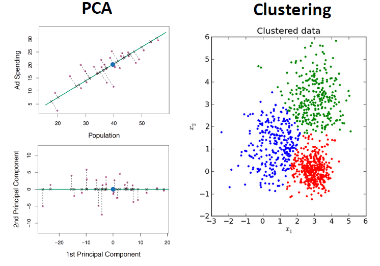
How are PCA and Clustering leading to less information? Consider a dataset.
What are the benefits?
Clustering References
https://en.wikipedia.org/wiki/K-means_clustering
https://en.wikipedia.org/wiki/K-means%2B%2B - kmeans++
https://www.youtube.com/watch?v=IuRb3y8qKX4 - video with visualization of training progress
https://www.youtube.com/watch?v=cWSnFaSjgBU - more on visualization
http://scikit-learn.org/stable/modules/generated/sklearn.cluster.KMeans.html
Marketing Motivation
You want to make a certain number of products for a large population of customers. We know a number of features describing each of the customers, and are able to target a product to a certain customer profile.
E.g.: different customers prefer cars which are fast, or get good gas mileage, or are cheap, or are luxurious and presigious (i.e., expensive), or are big, or are little, etc. And in various combinations.
The customers vary widely so we wish to make k products which cover as closely as possible what as many as possible customers would like.
The better you can do this, the better your products will sell.
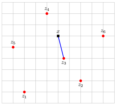
K-means clustering
- K clusters, centers are the means of cluster members.
- Each sample belongs to the cluster who's mean is nearest.
- Iteratively recompute membership and means (greedy optimization)
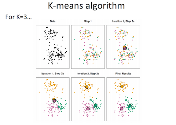
K-means algorithm
- Assign a number from 1 to K to each of N data points randomly
- While cluster assignments keep changing:
- For each of K clusters:
- Calculate cluster centroid
- For each of N points:
- Assign point to centroid it is closest to
- For each of K clusters:
Consider the possible ways to vary details in this method? How many clusters? How calculate distance?
k-Means as Greedy Optimization
The sum of all distances between members of a cluster gives a total length (a squared length can be viewed as a measure of "energy").
Within-Cluster-Variation: $WCV(C_k) = \dfrac{1}{|C_k|}\sum_{i, j \in C_k}d(x_{i}-x_{j})$, where $d(x_{i}-x_{j})$ is a distance metric of your choice.
k-means tries to minimize the net lengths over all clusters.
If you plotted this for each iteration, what would the plot look like?
Lab
Implement k-means clustering algorithm using scikit on IRIS, MNIST datasets.
Compute the net WCV for various options.
Look at result and WCV with different initializations.
Try varying the metric used in the clustering.
Vary k and plot WCV versus k.