BDS 761: Data Science and Machine Learning I

Topic 8: Embeddings

This topic:

0. Eigendecomposition review
1. Dimensionality Reduction & PCA
2. Graph Embedding
3. Information & t-SNE
4. Text Embedding
5. Neural Embeddings

Reading:

• Probabilistic Machine Learning: An Introduction, Murphy 2022, Ch 20. Dimensionality Reduction. https://probml.github.io/pml-book/book1.html
• J&M Chapter 5. Embeddings, https://web.stanford.edu/~jurafsky/slp3/
• https://scikit-learn.org/1.5/modules/manifold.html

Embedding intro

ELI5: Embedding

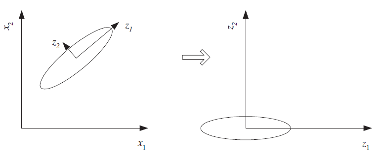
An embedding takes a longer vector (i.e., in high dimensions) and assigns to it a shorter vector (i.e. in a lower dimensional space), in a way that hopefully preserves the important variation, while discarding unimportant, redundant, or mostly-constant dimensions

$$\begin{pmatrix}v_1 \\ v_2 \\ v_3 \\ v_4 \\ \vdots \\ v_n \end{pmatrix} \rightarrow \begin{pmatrix}w_1\\ w_2 \\ \vdots \\ w_m \end{pmatrix} $$

There are many different approaches, ranging from very-simple to very involved.

Dimensionality Reduction - an older, broader field of methods

What if we want to embed things that aren't vectors, like categorical variables?

How could we embed text?

Data embedding

Recall these 2D data correlation plots.

The points can be seen as approximately on a lower dimensional manifold.

This is embedded in the higher dimensional space of the plot.

What is the dimensions of the manifolds? How would we represent a point on them?

Famous Matrices: Diagonal matrix

$$\mathbf D = \begin{bmatrix} D_{1,1} & 0 & 0\\ 0 & D_{2,2} & 0 \\ 0 & 0 & D_{3,3}\\ \end{bmatrix}$$

Consider what it implies for a linear system with a diagonal matrix.

Can completely describe with a vector $\mathbf d$ with $d_i = D_{i,i}$

Hence we write "$\mathbf D = \text{diag}(\mathbf d)$" and "$\mathbf d = \text{diag}(\mathbf D)$"

Relate to Hadamard product of vectors $\mathbf D \mathbf v = \mathbf d \odot \mathbf v$.

Famous Matrices: Diagonal matrix - Applications

1. Consider product $\mathbf D \mathbf v$

2. Consider products $\mathbf D \mathbf A$ and $\mathbf A \mathbf D$

3. Consider norm $\Vert \mathbf D \mathbf v \Vert_2$

4. Consider $\mathbf D_1 \mathbf D_2$

5. Consider power $\mathbf D^n$

6. Consider inverse of diagonal matrix $\bf D$

7. Solve linear system $\mathbf A \mathbf x = \mathbf b$ when $\mathbf A$ is diagonal.

Famous Matrices: Orthogonal matrix

Square marix where columns are orthogonal, i.e. $\mathbf a_i^T \mathbf a_j = 0$ when $i \ne j$

Orthonormal matrix $\rightarrow$ also have $\mathbf a_i^T \mathbf a_i = 1$

Famous Matrices: Orthogonal matrix - Applications

Geometrically, orthonormal matrices implement rotations.

Very easy inverse

Solve linear system $\mathbf U \mathbf x = \mathbf b$ for $\mathbf x$ when $\mathbf U$ is orthonormal.

Solve matrix system $\mathbf U \mathbf A = \mathbf V$ for $\mathbf A$ when $\mathbf U$ is orthonormal.

I = np.eye(5)
print(I)

[[1. 0. 0. 0. 0.]
 [0. 1. 0. 0. 0.]
 [0. 0. 1. 0. 0.]
 [0. 0. 0. 1. 0.]
 [0. 0. 0. 0. 1.]]

e0 = I[:,0]

print(e0)

[1. 0. 0. 0. 0.]

e0 = I[0,:]

print(e0)

[1. 0. 0. 0. 0.]

np.linalg.inv(D)*D

array([[1., 0., 0., 0.],
       [0., 1., 0., 0.],
       [0., 0., 1., 0.],
       [0., 0., 0., 1.]])

theta = 45*np.pi/180

R = np.array([[np.cos(theta), np.sin(theta)],[-np.sin(theta),np.cos(theta)]])
print(R)

[[ 0.70710678  0.70710678]
 [-0.70710678  0.70710678]]

R@np.array([0,1])

array([0.70710678, 0.70710678])

R@R.T

array([[ 1.00000000e+00, -4.26642159e-17],
       [-4.26642159e-17,  1.00000000e+00]])

Eigendecomposition

Reconsider: $${\bf A}{\bf u} = \lambda {\bf u}$$

IF $\mathbf A$ is $n \times n$ symmetric and real, we can find $n$ eigenvectors $\{ \mathbf u_i \}$ with corresponding real eigenvalues $\lambda_i$, i.e.

$${\bf A}{\bf u_i} = \lambda_i {\bf u_i}$$

If the eigenvalues are distinct, the eigenvalues are orthogonal. Otherwise they may not be orthogonal but are still linearly independent, so we can make an orthogonal basis.

Write this as ${\bf A}{\bf U} = $ ?

Diagonalization

a.k.a. Eigendecomposition

a.k.a. Spectral Decomposition)

$$ {\bf A}{\bf U} = {\bf U} \boldsymbol\Lambda \rightarrow {\bf A} = {\bf U} \boldsymbol\Lambda {\bf U}^{-1} $$

We can also solve for $\boldsymbol\Lambda$ = ?

Famous Matrices: Normal matrix

A real matrix $\bf A$ is a normal matrix if:

$$ \mathbf A \mathbf A^T = \mathbf A^T \mathbf A$$

Note this must be a square matrix due to matrix multiplication rules.

Examples of Normal matrices:

1. $\mathbf A = \mathbf B \mathbf B^T$ for some $m \times n$ matrix $\bf B$

2. $\mathbf A = \mathbf B^T \mathbf B$ for some $m \times n$ matrix $\bf B$

Famous Matrices: Normal matrix - value

If a real matrix $\bf A$ is a normal matrix then its eigenvectors are orthonormal.

$$ {\bf A}{\bf U} = {\bf U} \boldsymbol\Lambda \rightarrow ? $$

2D Normal Distribution

Consider how to construct these using independent 1D Normal distributions.

Exercise:

• Compute eigenvalue decomposition on covariance matrix for a dataset and identify eigenvalues and eigenvectors.
• Demonstrate ability to reassemble matrix from components.
• Assemble low rank approximation and visualize difference.

Dimensionality Reduction

Dimensionality Reduction - Motivation

1. Reducting problem complexity. Complexity of any classifier or regressor depends on the number of inputs.
   1. time and space complexity
   2. necessary number of training examples to train such a classifier or regressor.
   3. Curse of dimensionality
2. Visualization - 2D retina, 3D mental capacity, $n$-dimensional data

Feature selection - choose a subset of important features pruning the rest

Feature extraction - form fewer, new features from the original inputs

Features for dim reduction

1. Feature selection - given $d$ inputs, choose $k<d$ inputs to keep, discard the rest.
2. Feature extraction - compute $k<d$ new inputs using combinations of original inputs. E.g. replace multiple inputs with their average.

Feature extraction: Linear Methods

Here, linear means new features are linear combinations of original features. E.g. mean of multiple features.

• Principal Component Analysis (PCA) - use SVD & keep singular vectors for largest singular values

• Linear Discriminant Analysis (LDA) - supervised variation on PCA

• Factor Analysis -

• Multidimensional Scaling -

• Canonical correlation analysis - finds joint features that relate multiple datasets

Exercise:

write the SVD of your dataset and identify the combinations of original inputs

create low-rank approximations to your data covariance matrix and visualize how similar they are.

Principal Component Analysis

1. Center the data

2. Rotate axes to line up directions of highest variance

Principal Component Analysis

Using eigendecomposition to identify embedding spaces, dimensions

1. remove means
2. compute covariance matrix
3. compute eigenvalues

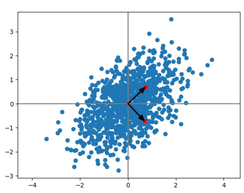
https://medium.com/intuition/mathematical-understanding-of-principal-component-analysis-6c761004c2f8

Exercise: Consider the application of this to your 2D Normal distributions.

Scree graph

plot of variance explained as a function of the number of eigenvectors kept

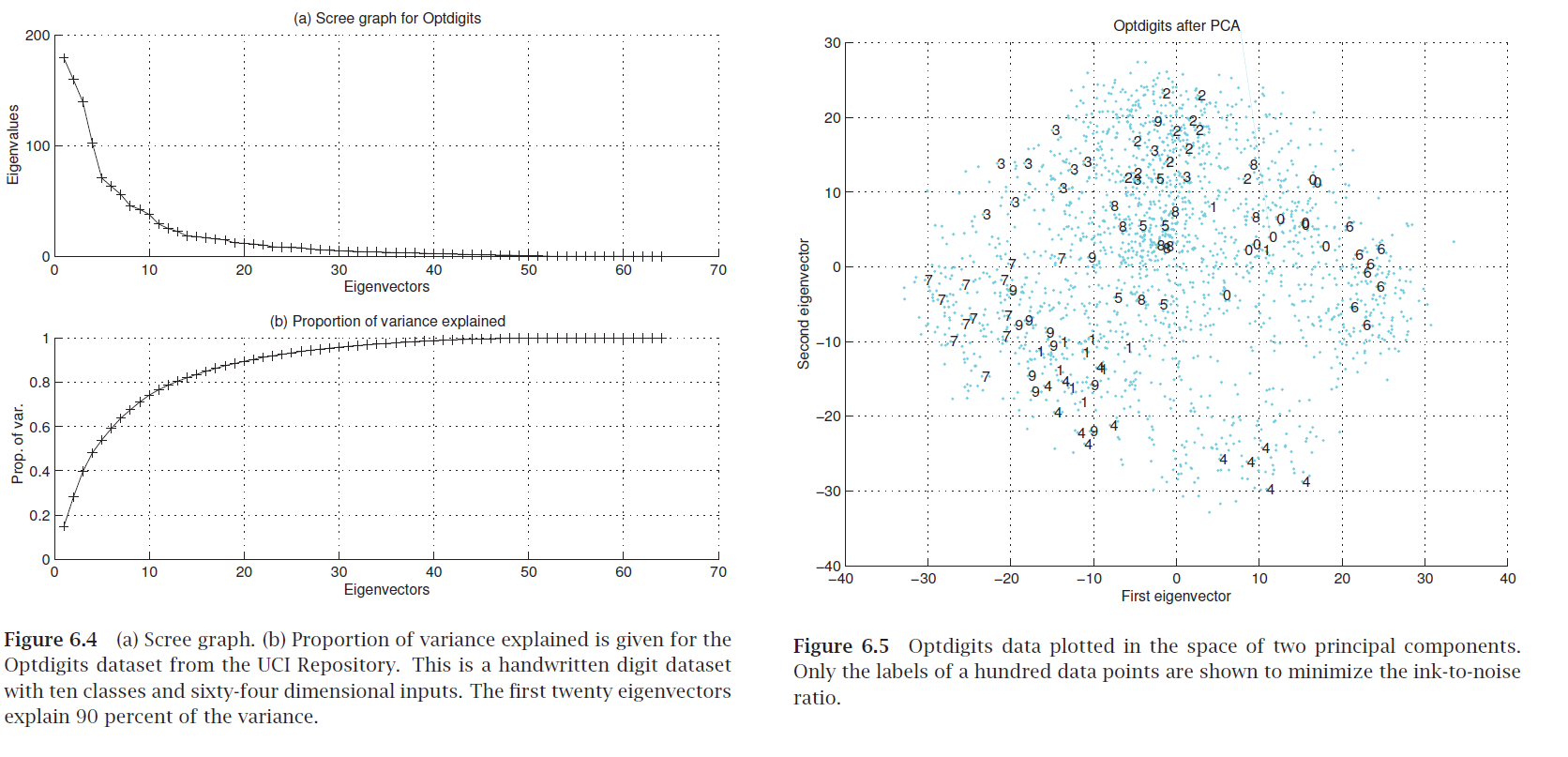
Exercise: how do you compute "variance explained"?

"Eigendigits" = eigenvectors of handwritten digit image dataset (with images as rows).

Exercise 2: what are the original and extracted features in the geometric figure?

Exercise:

Using a sklearn classification dataset, compute the Scree graph.

Use the PCA function in sklearn to embed the data in 2D and make a scatterplot with different colors for the different classes.

Graph Embedding

Network Embedding versus "Data Embedding"

Note when dealing with network methods we have two possible starting points:

1. Starting with an already-made network (given an adjacency matrix describing connections between a set of nodes)
2. Starting with a dataset (given a matrix of samples versus features), where the first step is to form the network (somehow)

In #2, we start with a set of sample vectors, then compute a bunch of embedded model locations, which might be viewed as new sample vectors (now in a lower number of dimensions).

What are other names used for approach #2?

Aside: Mean-removal matrix $H$

Note that we can perform mean-removal for a matrix using linear algebra as

\begin{align} \bar{X} &= X - \tfrac{1}{n}\mathbf{1}\mathbf{1}^\top X \\ &= (I - \tfrac{1}{n}\mathbf{1}\mathbf{1}^\top ) X \\ &= HX \end{align}

where $\bar{X}$ as is $X$ with means removed and $H = I - \tfrac{1}{n}\mathbf{1}\mathbf{1}^\top$.

Note that $H$ is a projection matrix, and $H^T H = H H = H$

PCA

We can compute the mean-removed sample covariance matrix as: $ C = \tfrac{1}{n} X^\top H X. $

Solve eigenvectors $Cu=\lambda u$ for largest eigenvalues $\lambda$.

Embedding: principal component scores $X_c u$.

Classical MDS

Multidimensional Scaling

Use Euclidean distance matrix, with row-means removed: $ B = -\tfrac12 H D^{(2)} H,$

Solve $Bv=\lambda v$.

Use top $k$ eigenpairs for embedding.

Spectral Graph theory

Key here is instead of a data matrix of vectors we have an adjacency (or related) matrix of similarities

Consider how the covariance matrix from PCA contains both weak correlations and strongs ones.

With spectral embeddings, we basically truncate the small ones using asimilarity score or binary threshold, allowing long-range nonlinear variation, but maintaining locally linear relationships.

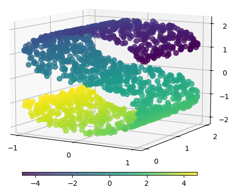
Spectral clustering

Combine the nonlinear manifold embedding with clustering

https://scikit-learn.org/1.5/auto_examples/cluster/plot_cluster_comparison.html#sphx-glr-auto-examples-cluster-plot-cluster-comparison-py

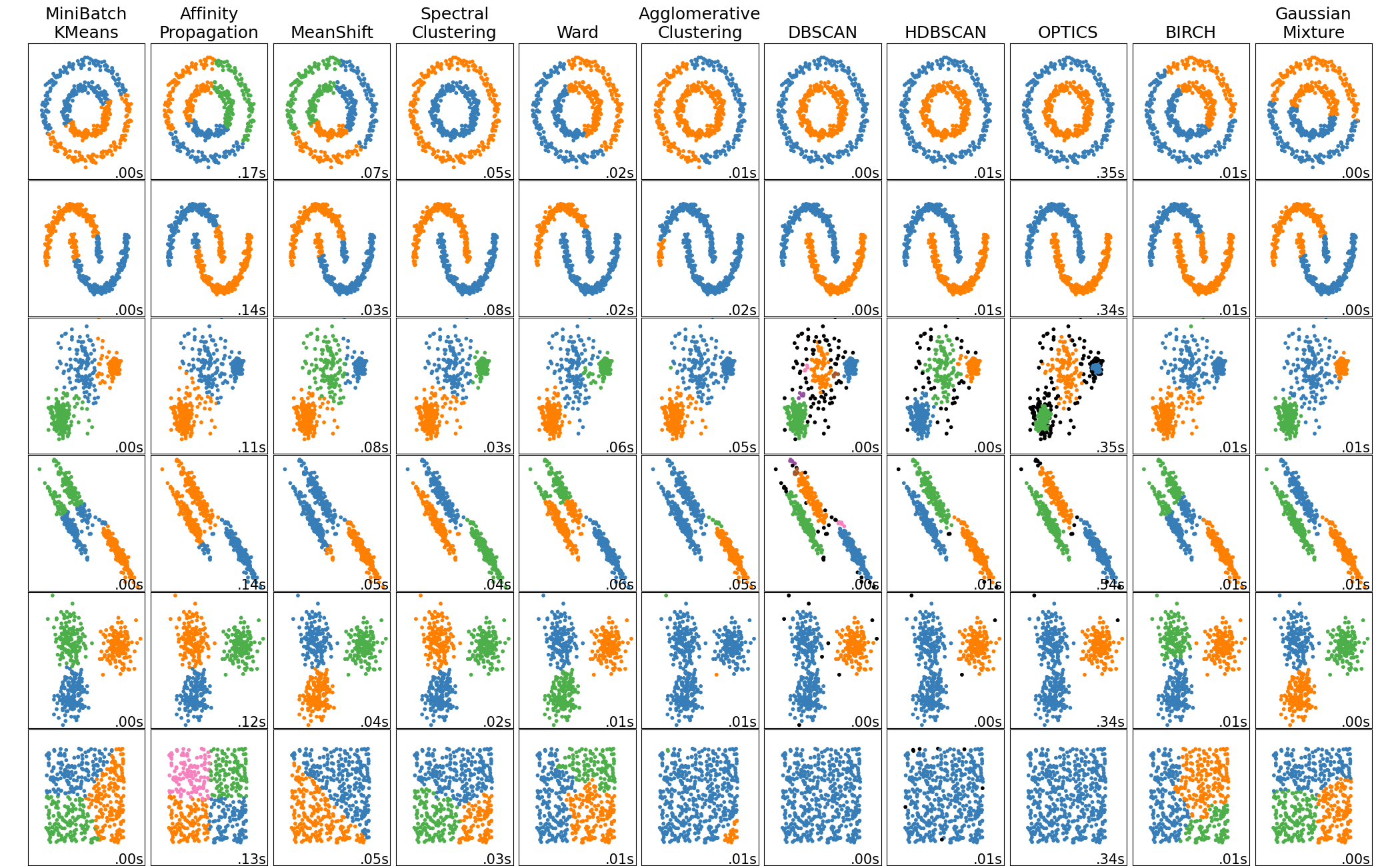
View as distances within the manifold used to cluster,rather than Euclidean distancs

Isomap

Matrix: same $B$ as MDS but with geodesic distances from shortest paths $d_{ij}$.

Apply classical MDS to $d_{ij}$

Diffusion Maps

Given a weighted adjacency matrix $W$ with degree matrix $D$,

Form matrix: $ P = D^{-1}W $ or symmetric $ K = D^{-1/2} W D^{-1/2} $.

Solve $P v = \lambda v$ or $K v = \lambda v$.

Use top $k$ eigenpairs for embedding.

Spectral Clustering (Normalized Cut)

Matrix: $ L_{\mathrm{sym}} = I - D^{-1/2} W D^{-1/2}. $

Solve $L_{\mathrm{sym}} v = \lambda v$.

Use eigenvectors with smallest nonzero eigenvalues.

Equivalently use eigenvectors for largest eigenvelues of $D^{-1/2} W D^{-1/2}$, similar to other methods.

In spectral clustering, we subsequently cluster these embedded points.

Laplacian Eigenmaps

Matrix: $ L = D - W $ or generalized $ L v = \lambda D v $.

Solve $Lv=\lambda Dv$.

Use eigenvectors with smallest nonzero eigenvalues.

Note that if $D$ is constant (all node degrees same) then we get the same eigenvectors as if we used the maximum eigenvalues of $W$ itself.

Graph Laplacians - graph version of Laplace operator $\nabla^2$ (average 2nd derivative over all coordinates)

Unnormalized - binary graphs: $ \mathbf L = \mathbf D - \mathbf A $, weighted graphs: $ \mathbf L = \mathbf D - \mathbf W $

Symmetric: $ \mathbf L_{sym} = \mathbf D^{-\frac{1}{2}} \mathbf L \mathbf D^{-\frac{1}{2}} $

Random walk: $ \mathbf L_{rw} = \mathbf D^{-1} \mathbf L $

Scikit-Learn Manifold Learning methods

https://scikit-learn.org/stable/auto_examples/manifold/plot_compare_methods.html#sphx-glr-auto-examples-manifold-plot-compare-methods-py

t-SNE

KL Divergence

Quick Information Theory review

For a discrete random variable $X$ with possible outcomes $x_i$ that have probabilities $p_i$, the information in an outcome measurement which gives $x_i$ is:

$$ I(x_i) = -\log_2 P(X=x_i) = -\sum_i p_i \log_2 p_i, $$

Consider an event which is 8 independent coin flips of a fair coin resulting in 10110101.

Entropy is the expected value over all possible outcomes:

$$ H(X) = -\sum_i P(X=x_i) \log_2 P(X=x_i) = -\sum_i p_i \log_2 p_i. $$

Perplexity is the effective number of outcomes from some average information. E.g. if coin was fair.

$$ \text{Perp}(P) = 2^{H(P)}$$

How does this fit the previous example?

K-L Divergence

Kullback–Leibler (K-L) divergence measures how one probability distribution $Q(x)$ diverges from another $P(x)$ that represents the “true” or reference distribution. For the discrete case: $$ D_{KL}(P \parallel Q) = \sum_i P(X=x_i) \log \frac{P(X=x_i)}{Q(X=x_i)} $$

How does the K-L Divergence relate to the information?

K-L divergence notes

We write it simply as $$ D_{KL}(P \parallel Q) = \sum_x P(x) \log \frac{P(x)}{Q(x)} $$

• Think of $P$ as the real data distribution.
• $ Q$ is your model or approximation.
• $D_{KL}(P|Q)$ quantifies the “extra information” or inefficiency (in bits) when encoding data from $P$ using a code optimized for $Q$ instead of $P$.
• It is non-negative and equals 0 only when $P(x) = Q(x)$ for all $x$. So similar to a distance metric.
• However it is not symmetric, so $D_{KL}(P|Q) \neq D_{KL}(Q|P)$ in general.

Example

Suppose a biased coin actually has $$ P(\text{Heads}) = 0.9,\quad P(\text{Tails}) = 0.1 $$ but your model assumes $$ Q(\text{Heads}) = 0.5,\quad Q(\text{Tails}) = 0.5 $$ Then: $$ \begin{aligned} D_{KL}(P|Q) &= 0.9 \log_2\frac{0.9}{0.5} + 0.1 \log_2\frac{0.1}{0.5} \ &\approx 0.9(0.85) + 0.1(-2.32) = 0.603\ \text{bits.} \end{aligned} $$

So, on average, you need 0.6 extra bits per flip to encode the true outcomes if you use the wrong model.

t-SNE

"(Student-) t-distributed Stochastic Neighbor Embedding"

Targets 2D or 3D embeddings for visualization

Balances local and global structure by minimizing K-L Divergence between distribution for each.

https://scikit-learn.org/stable/modules/generated/sklearn.manifold.TSNE.html

"Visualizing High-Dimensional Data Using t-SNE", van der Maaten and Hinton, JMLR 2008.

t-SNE Algorithm

For points $x_i\in\mathbb{R}^D$:

Model high-dimensional similarities with Gaussian kernels $$ p_{j|i}=\frac{\exp(-|x_i-x_j|^2/2\sigma_i^2)}{\sum_{k\neq i}\exp(-|x_i-x_k|^2/2\sigma_i^2)} $$

Choose desired Perp of $p_{j|i}$ as input parameter, and $\sigma_i^2$ is chosen to achieve this. Then for symmetrized distribution:

$$ p_{ij}=\frac{p_{i|j}+p_{j|i}}{2N}. $$

Model low-dimensional similarities for embedded points $y_i\in\mathbb{R}^2$ using Student-t kernels $$ q_{ij}=\frac{(1+|y_i-y_j|^2)^{-1}}{\sum_{k\neq l}(1+|y_k-y_l|^2)^{-1}}. $$

Student-t distribution has heavy tails to avoid overly-clustering data. Also convenient choice for optimization complexity.

Optimize over embedded points by minimizing KL divergence between these distributions. $$ \mathrm{KL}(P|Q)=\sum_{i\neq j} p_{ij}\log\frac{p_{ij}}{q_{ij}}. $$

from sklearn.manifold import TSNE
#help(TSNE)

import numpy as np
from sklearn.manifold import TSNE
import matplotlib.pyplot as plt

# toy dataset: three tight clusters in 2D, then embedded to 10D
rng = np.random.default_rng(0)
A = rng.normal([0,0], 0.1, (50,2))
B = rng.normal([3,0], 0.1, (50,2))
C = rng.normal([0,3], 0.1, (50,2))
X2 = np.vstack([A,B,C])

# map to 10D with a random linear transform
W = rng.normal(size=(2,10))
X10 = X2 @ W

# t-SNE back to 2D
Y = TSNE(n_components=2, perplexity=20, learning_rate=200, init="random", random_state=0).fit_transform(X10)

plt.figure(figsize=(3,3))
plt.scatter(Y[:,0], Y[:,1], c=np.repeat([0,1,2], 50), s=20)
plt.title("Toy t-SNE example")
plt.show()

Exercise: Apply to your classification dataset. Try varying the complexity.

Text embedding methods

Topic Modeling

• Determine small set of topics for corpus of documents, e.g. politics, art, sports
• Unsupervised learning problem - factor word-document matrix - SVD, NNMF, Latent Dirichlet Allocation

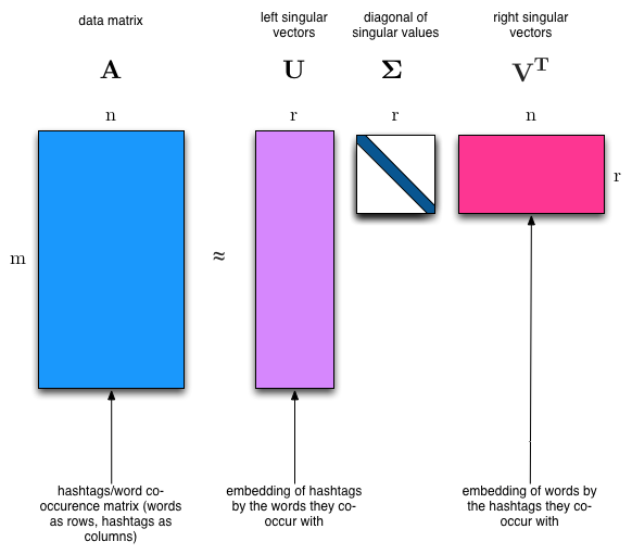
Matrix Factorization

Break matrix into two or more $\mathbf X = \mathbf F \mathbf G$

Analogous to factoring a number, e.g. $28 = 7 \times 2 \times 2$

If $\mathbf X$ is $N \times d$, what are sizes of factors?

$\mathbf G$ as factors in terms of original features

$\mathbf F$ as samples transformed to factor combinations

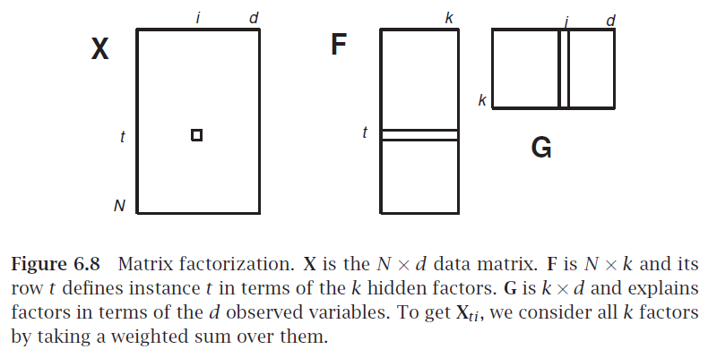
How could we use the SVD for this?

Latent Semantic Indexing

$\mathbf X$ is a sample of $N$ documents each using a bag of words representation with $d$ words

each factor may be one topic or concept written using a certain subset of words

each document is a certain combination of such factors

$\mathbf G$ relates documents to factors

$\mathbf F$ relates words to factors

Application: Recommender System

We have $N$ customers and we sell $d$ different products

$X_{ij}$ is number of times customer $i$ bought product $d$

$\mathbf G$ relates customers to factors

$\mathbf F$ relates products to factors

...point of these is to get some new customer or document and compute something. But what?

Word embeddings

Word embedding - Motivation

Most machine learning methods are based on numerical mathematical mathods which operate on vectors of numbers. E.g. deep learning.

But when text is converted to numbers via most common approaches, the numbers are not very meaningful.

Example of meaningful vectors:

• array of light levels in image
• list of concentration levels of chemicals

Example of less-meaningful vectors:

• list of base-pairs in DNA converted to 0,1,2,3
• list of ascii code of letters in document

Goal: Convert text into vectors who's geometric locations are meaningful. So similar text passages have similar vectors

Distributional hypothesis

Words that occur in similar contexts tend to have similar meanings.... so close together in a gometric sense.

Synonyms (like oculist and eye-doctor) tended to occur in the same environment (e.g., near words like eye or examined) with the amount of meaning difference between two words “corresponding roughly to the amount of difference in their environments” (Harris, 1954, 157).

Do you agree with this? Or is there more information besides that described by a word's context?

Word embedding

What might the manifold for word "relatedness" look like?

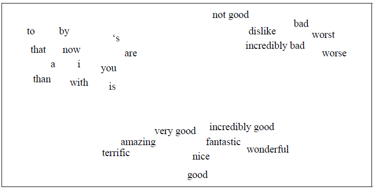
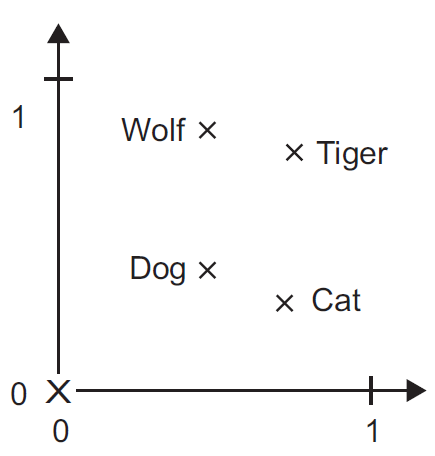
Figure 6.1 A two-dimensional (t-SNE) projection of embeddings for some words and phrases, showing that words with similar meanings are nearby in space. The original 60- dimensional embeddings were trained for a sentiment analysis task. Simplified from Li et al. (2015).

Vector semantic models

• Embeddings of word in a particular vector space
• Better handle OOV words, only need similar words in training set
• Can be learned automatically from text without any complex labeling or supervision.
• Now the standard way to represent the meaning of words in NLP

Will cover two models: tf-idf and word2vec

Term-document matrix

A kind of co-occurence matrix, which counts how ofen words co-occur based on being in the same context or document. BOW representation of documents.

Figure 6.2 The term-document matrix for four words in four Shakespeare plays. Each cell contains the number of times the (row) word occurs in the (column) document.

Dimensionality of vectors is number of words used, here 4. Equal to vocabulary size used.

Gigantic matrix for all words $\times$ all documents. Exploit sparsity.

Document vectors

Used in Information Retrieval field. Document search based on vector similarity to search term.

Figure 6.3 The term-document matrix for four words in four Shakespeare plays. The red boxes show that each document is represented as a column vector of length four.

Perform search by putting search query into vector and computing a distance metric with document vectors.

Word vectors

Use rows of matrix to compare vectors

More common to use word-word matrix, a.k.a term-term matrix or term-context matrix.

Numbers are counts of times the two words appear together in same context: same document, or a sliding window within documents.

Note similarity of rows for information and digital, and of rows for apricot and pineapple.

Exercise: compute cosine similarity between Apricot, Digital, and Information.

Dense Embeddings

Two-step process:

1. Convert text to numbers via simple approach
2. Dimensionality reduction

Wide range of Embedding methods

• Principal component analysis & related methods applied to BOW data ~ Latent semantic indexing
• GloVe - Dim reduction on matrix of co-occurence statistics.
• Shallow neural network layer - Embedding layer
  • Neural embedding: word2vec, doc2vec, x2vec

GloVe - Global Vectors for Word Representation

Can download and use result: https://nlp.stanford.edu/projects/glove/

Neural word embeddings

Embedding via linear layer

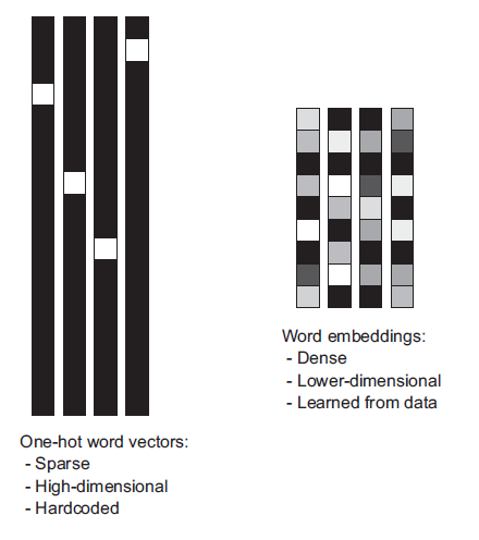
One-hot encoding converts words (or $n$-grams) into orthogonal vectors $\mathbf e_k$ with a single "1" value and the rest zeros. Vectors for any two words are orthogonal. So to handle 50,000 words requires length-50,000 vectors.

Geometrically these are orthogonal vectors in 50,000-dimensional space. With every word vector equally-distant from every other.

Word embeddings have a much smaller number of output dimensions.

Can use any word embedding we have previously covered here.

Exercise - Embedding Layer

1. Draw a dense linear single-layer network with no activation function, with $N$ inputs and $m$ outputs,

2. write the output for a one-hot encoded input vector $\mathbf e_k$ representing a single word.

3. write the output for a general input vector $\mathbf v$ representing multiple words in a document.

word2vec

general idea: model probability of both target word with context.

“Is word w likely to show up near apricot?”

Use running text as implicitly supervised training data

• no need for hand-labeling
• Bengio 2003 and Collobert 2011 used for neural language model

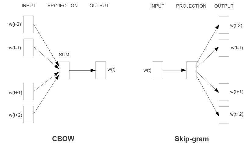
word2vec contains two algorithms:

1. Continuous Skip-gram - predict neighboring words of given word
2. Continuous bag-of-words (CBOW) - predict target word given neighbors

Continuous = dense embedding vector rather than sparse binary.

Negative Sampling = minimize the log-likelihood of those randomly-chosen other words from lexicon. "Skip-gram with Negative Sampling (SGNS)"

Can download and use result: https://code.google.com/archive/p/word2vec

The classifier

Given tuple of words $(t,c)$, e.g. $(apricot,jam)$:

• $t$ = target word
• $c$ = candidate context word

Predict $P(+|t,c)$ probability $c$ is a context word.

Probability $c$ is not a context word: $P(-|t,c) = 1- P(+|t,c)$

Classifier model - basically just a similarity metric, made into probability by sigmoid function.

\begin{align} P(+|t,c) &= \sigma(\text{"similarity"}) \\ &= \frac{1}{1-e^{-\mathbf t \cdot \mathbf c}} \end{align}

where $\mathbf t$ and $\mathbf c$ are the dense vectors representing the words -- these are the parameters of the model which we will fit using data.

\begin{align} P(-|t,c) &= 1-P(+|t,c) \\ &= \frac{e^{-\mathbf t \cdot \mathbf c}}{1-e^{-\mathbf t \cdot \mathbf c}} \end{align}

"skip-gram"

A variation on a bigram which combines target word and context word (not necessarily neighbor), hence it "skips" other context words.

Context words assumed independent of each other, so for a target word and list of context words,

\begin{align} P(+|t,(c_1, c_2,...)) &= \prod_i \frac{1}{1-e^{-\mathbf t \cdot \mathbf c_i}} \end{align}

Bigrams:

• $t$ and immediately preceding word
• $t$ and immediately following word

Skip-grams:

• $t$ and word two words away
• $t$ and word three words away
• ...

Examples:

Hyperparameter: ratio between numbers of positive and negative examples $k$ (=2 above)

Semantic Properties of Embeddings

context window size

• small window - semantically-similar words, same parts of speech
• large window - topically related words, not similar

First order co-occurence (syntagmatic association) - words typically near each other. $wrote$ and $book$

Second-order co-occurrence (paradigmatic association) - have similar neighbors $wrote$ and $said$

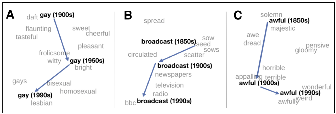
Relational meanings (analogous meanings) via word differences: $king-man+woman = queen$

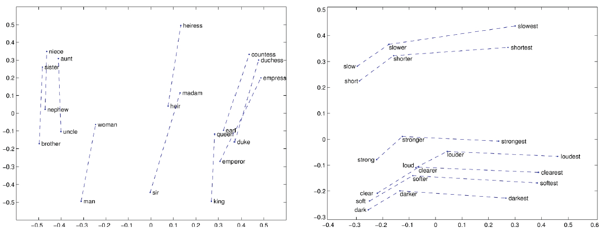
• gender vector
• comparative & superlative morphology
• temporal changes
• bias: $doctor-man+woman = nurse$

Neural Representations

Deep Learning Models for Representation

• Called representation learning models and their outputs are learned representations or learned feature representations
• Called Neural embedding or learned embedding in NLP
• Not embeddings in the classical sense; do not preserve topology or injectivity.
• Produce a vector-space structure that provides task-relevant similarity/separation.
• can be specially trained for embedding use, or based on task-trained model.

Motivation: Vector databases

Vector databases store and index embedding vectors $$ z \in \mathbb{R}^d $$

They support fast approximate similarity search as $\operatorname{arg,min}_{i\in \mathcal I} d(z_q, z_i)$, typically using cosine or $\ell_2$ distance.

Embeddings from LLMs other large models enable semantic search, retrieval-augmented generation, clustering, and deduplication between practically anything, at scale.

support finding the nearest neighbors of an embedded query vector efficiently when datasets can have $10^{10}$ vectors.

https://aws.amazon.com/what-is/vector-databases/, https://www.ibm.com/think/topics/vector-database

Indexing methods - basic, efficient, scalable

Quantization methods - Split the space and compress vectors.

• Product Quantization (PQ)
• Optimized Product Quantization (OPQ)
• Residual Quantization

Graph-based indexes - build a proximity graph and search along it.

• HNSW (Hierarchical Navigable Small World)
• NSG, KGraph

Tree / partition methods

• KD-trees (small d only)
• Randomized trees
• Annoy (forest of random projection trees)

Examples

• FAISS (Meta): the foundational ANN library; provides PQ, OPQ, IVF, HNSW. https://github.com/facebookresearch/faiss
• Annoy (Spotify): lightweight, tree-based, good for read-heavy workloads.
• HNSWlib: pure HNSW implementation, state-of-the-art graph search.
• ScaNN (Google): optimized for TPUs and cosine similarity.
• Milvus: full database with clustering, partitions, dynamic updates. https://milvus.io/
• Weaviate: vector-native DB with metadata filters and schema.
• Pinecone: managed service built on graph + quantization hybrids.
• Elasticsearch / OpenSearch vector search: integrates ANN into traditional IR.

Handle various trade-offs and features differently

Deep Learning for Embedded Representations

The first layer of a modern LLM is a linear layer called the Embedding layer, which convert tokens (view as one-hot encoded) into shorter dense representations (e.g. length 1024). these are not the embeddings we are talking about here.

The output of a LLM are the logits (result of softmax) used to predict a word.

The representation used for downstream tasks and for embeddings is the layer before that. View the softmax as a classifier, the learned representation is the values that are to be classified.

The shape of this output is often not desired, so some technique called pooling is used to average over it partially.

Representations can similarly be extracted using CNN's and other types of architectures.

Sentence Transformers Framework

Canned framework for sentence, text and image embeddings.

https://www.sbert.net/

https://huggingface.co/sentence-transformers

# pip install sentence-transformers

from sentence_transformers import SentenceTransformer, util

model = SentenceTransformer("sentence-transformers/all-MiniLM-L6-v2")
s1 = "The patient has diabetic retinopathy."
s2 = "The eye shows signs of retinal damage."

v1 = model.encode([s1])
v2 = model.encode([s2])
v1.shape

(1, 384)

plt.figure(figsize=(5,3))
plt.plot(v1.flatten());
plt.plot(v2.flatten());

sim = util.cos_sim(v1, v2)
print(sim.item())

0.5058673024177551

s3 = "I ate pasta for lunch."
v3 = model.encode([s3])
sim = util.cos_sim(v1, v3)
print(sim.item())

0.02934318035840988

Manually using a Model

Recall the pipeline, have to tokenize input ourself

then convert output to a vector.

import torch
from transformers import AutoTokenizer, AutoModel
from sklearn.metrics.pairwise import cosine_similarity

# CHOOSE ONE:
MODEL_NAME = "bert-base-uncased"
# MODEL_NAME = "roberta-base"
# MODEL_NAME = "distilbert-base-uncased"
# MODEL_NAME = "microsoft/deberta-v3-base"
#MODEL_NAME = "roberta-base"

tok = AutoTokenizer.from_pretrained(MODEL_NAME)
model = AutoModel.from_pretrained(MODEL_NAME)
model.eval()

def embed_sentence(text: str, use_cls: bool = False) -> torch.Tensor:
    x = tok(text, return_tensors="pt", truncation=True, padding=True)
    with torch.no_grad():
        out = model(**x)
        hidden = out.last_hidden_state      # [1, T, H]

    if use_cls:
        # CLS pooling: first token
        emb = hidden[:, 0, :]              # [1, H]
    else:
        # mean pooling over non-padding tokens
        mask = x["attention_mask"].unsqueeze(-1)  # [1, T, 1]
        masked = hidden * mask
        emb = masked.sum(dim=1) / mask.sum(dim=1)

    emb = emb / emb.norm(p=2, dim=-1, keepdim=True)
    return emb.squeeze(0)

s1 = "The patient has diabetic retinopathy."
s2 = "The eye shows signs of retinal damage."
s3 = "I ate pasta for lunch."

e1 = embed_sentence(s1, use_cls=False).numpy()
e2 = embed_sentence(s2, use_cls=False).numpy()
e3 = embed_sentence(s3, use_cls=False).numpy()

print("sim(s1, s2) =", cosine_similarity([e1],[e2])[0,0])
print("sim(s1, s3) =", cosine_similarity([e1],[e3])[0,0])

sim(s1, s2) = 0.75558174
sim(s1, s3) = 0.40877026

Image Embedding example

Image classifiers (i.e., CNN's) operate directly on image data.

Must convert output to a vector

from matplotlib import pyplot as plt
from sklearn.datasets import load_sample_image
flower = load_sample_image('flower.jpg') 
china = load_sample_image('china.jpg')   
plt.imshow(china);
plt.figure();
plt.imshow(flower);

china.shape

(427, 640, 3)

import numpy as np
import torch
from transformers import AutoImageProcessor, AutoModel

# HuggingFace CNN ResNet-50
model_name = "microsoft/resnet-50"
processor = AutoImageProcessor.from_pretrained(model_name)
model = AutoModel.from_pretrained(model_name)
model.eval()

def get_embedding(np_image: np.ndarray) -> np.ndarray:
    """
    np_image: H x W x 3 (RGB), uint8 or float32
    returns: 1D embedding as numpy array
    """
    inputs = processor(images=np_image, return_tensors="pt")
    with torch.no_grad():
        outputs = model(**inputs)                 # last_hidden_state: [1, C, H', W']
        feat_map = outputs.last_hidden_state
        emb = feat_map.mean(dim=[2, 3])           # global average pooling → [1, C]
        # L2-normalize
        emb = emb / emb.norm(p=2, dim=-1, keepdim=True)
    return emb.squeeze(0).cpu().numpy()          # shape (C,)

# Compute embeddings
e_flower1  = get_embedding(flower)
e_flower2  = get_embedding(np.flipud(flower))
e_china    = get_embedding(china)

flower.shape, np.prod(flower.shape), e_flower1.shape

((427, 640, 3), np.int64(819840), (2048,))

def cossim(v1,v2):
    return float(np.dot(v1,v2)/np.sqrt(np.dot(v1,v1))/np.sqrt(np.dot(v2,v2)))

print(cossim(flower.flatten(),np.flipud(flower).flatten())), 
print(cossim(e_flower1,e_flower2))

0.04443359375
0.9064571857452393

print(cossim(flower.flatten(),china.flatten())), 
print(cossim(e_flower1,e_china))

0.513671875
0.2582722306251526