BDS 761: Data Science and Machine Learning I

def multivariate_normal(x, n, mean, cov):
    return (1./(np.sqrt((2*np.pi)**n * np.linalg.det(cov))) * np.exp(-1/2*(x - mean).T@np.linalg.inv(cov)@(x - mean)))


mean = np.array([35,70])
cov = 100*np.array([[1,.5],[.5,1]])
pic = np.zeros((100,100))
for x1 in np.arange(0,100):
    for x2 in np.arange(0,100):
        x = [x1,x2]
        pic[x1,x2] = multivariate_normal(x, 2, mean, cov)

figure(figsize=(4,3))
contour(pic);
grid();
print(cov)
[[100.  50.]
 [ 50. 100.]]

from scipy.stats import multivariate_normal
mu = np.array([0., 0.])
sigma = np.eye(2)
x, y = np.mgrid[-1:1:.01, -1:1:.01]
pos = np.empty(x.shape + (2,))
pos[:, :, 0] = x; pos[:, :, 1] = y

rv = multivariate_normal(mu, sigma)

figure(figsize=(4,3))
contourf(x, y, rv.pdf(pos));
colorbar();

Generate 1000 1D random variables using numpy with mean 2 and standard deviations 3
Compare the theoretical distribution to the histogram of points
Joint distribution: $p(\text{temperature anomaly}, \text{$CO_2$ concentration})$
Correlations are useful, whether due to causality or a common cause
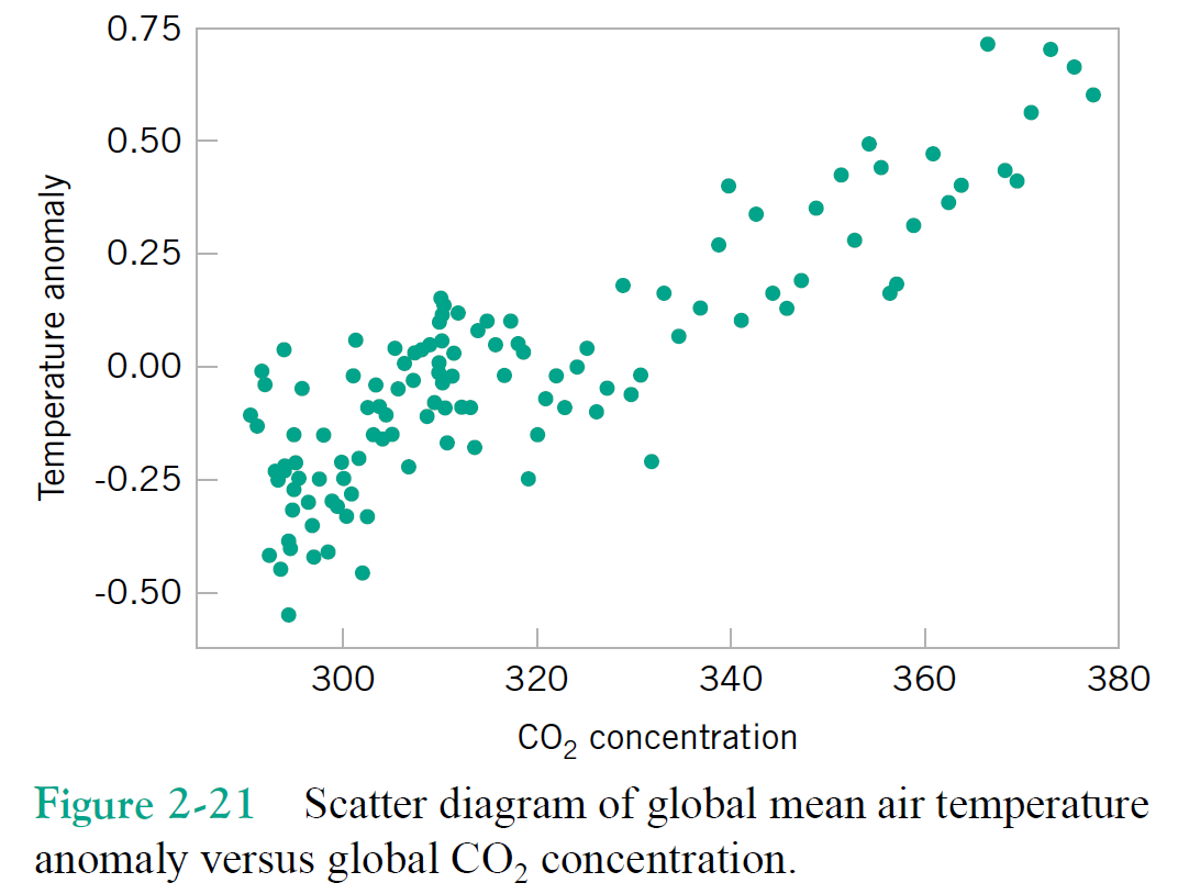
If I know the $CO_2$ concentration is over 400, what do I expect the temerature anomaly to be?
Generally given a $CO_2$ concentration of $x_i$, what is the corresponding temperature anomaly, "$y(x_i)$" (approximately)
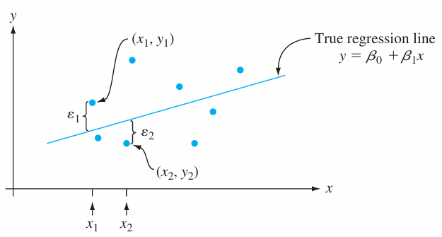
Choose to use a model of the form $y(x) = \beta_0 + \beta_1 x$, where $fitting$ refers to the choice of the best $\beta_0$ and $\beta_1$ -> choose slope and intercept
Two separate "functions" here: the probability distribution $p(x,y)$, and the regression model $\hat{y}(x_i) \approx y_i$
Devore, "Probability and Statistics for Engineering and the Sciences", Brooks. (2000).
in other words, \begin{align} x &= [0, 1,2,3,4,5,6,7] \\ y &= [3, 6,5,6,9,12,10,13] \end{align}
y = [3,6,5,6,9,12,10,13]; x = range(0,len(y))
figure(figsize=(6,2))
plot(x,y,'o'); grid(); xlabel('x'); ylabel('y');

Basically the model is saying $ y \approx \beta_0 + \beta_1 x$.
How approximate? Well the residual $\varepsilon = y - (\beta_0 + \beta_1 x)$ is presumed to be uninteresting random values ...so a statistical model is implied
E.g., zero-mean, Gaussian. Educated guesses? Are they correct?
We assume the data has a mean which varies with the dependent variable $x$
$$ \mathbb{E}[Y \ | \ X = x] = \beta_0 + \beta_1 x $$We further assume $\varepsilon = y - (\beta_0 + \beta_1 x)$, is normally distributed, and so
$$ P(Y \ | \ X=x) = \frac{1}{\sqrt{2\pi}\sigma} \exp\left\{\frac{-(y - (\beta_0 + \beta_1 x))^2}{2\sigma^2}\right\} $$This means the probability distribution over random variable $Y$ which takes values $Y = y$ with some probability, at the point in time when the random variable $X$ is presumed to be known to take the value $x$ (so not treated as random).
Find the parameters $\beta_0$ and $\beta_1$ in this model given some data:
$$ P(Y \ | \ X) = \frac{1}{\sqrt{2\pi}\sigma} e^{\frac{-(y - (\beta_0 + \beta_1 x))^2}{2\sigma^2}} \text{ for } -\infty < x < \infty $$Measurements are independent, so $P(Y_1,Y_2,...) = P(Y_1)P(Y_2)...$
Every measurement follows same distribution, here $ P(Y \ | \ X)$
We can choose convenient $x$ values since not treated as random (assuming we don't use this to cheat somehow)
Note relation to 2D Normal $P(X,Y) = P(Y|X)P(X)$
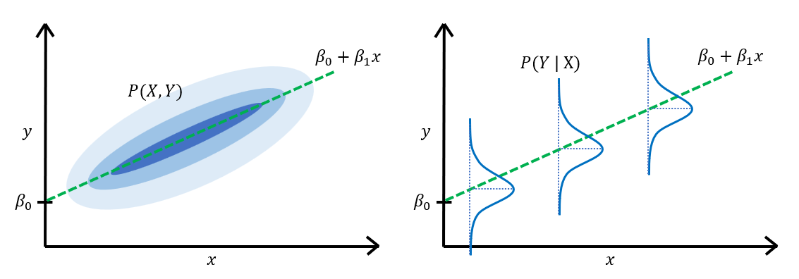
The likelihood for a model sample (a.k.a. dataset) is defined as the function of model parameters using the data
$$ L(\beta_0, \beta_1, \sigma^2) = \prod_{i=1}^{n} P(Y = y_i \ |\ X=x_i) = \prod_{i=1}^{n} \frac{1}{\sqrt{2\pi\sigma^2}} \exp\left(-\frac{(y_i - (\beta_0 + \beta_1 x_i))^2}{2\sigma^2}\right) $$Our goal is to choose the most likely parameters, meaning those which maximize the likelihood
$$ (\beta_0, \beta_1) = \arg \max_{\beta_0, \beta_1} L(\beta_0, \beta_1, \sigma^2) = \arg \max_{\beta_0, \beta_1}\prod_{i=1}^{n} \frac{1}{\sqrt{2\pi\sigma^2}} \exp\left(-\frac{(y_i - (\beta_0 + \beta_1 x_i))^2}{2\sigma^2}\right) $$since the distributions are all over different random variables, we get a multidimensional Normal distribution
Because we only want the argument, we don't care about the actual maximum value, just the choice of arguments which achieve the maximum.
Given that plus the fact that probabilities are always positive we can choose to maximize the log
$$ (\beta_0, \beta_1) = \arg \max_{\beta_0, \beta_1} L(\beta_0, \beta_1, \sigma^2) = \arg \max_{\beta_0, \beta_1} \log L(\beta_0, \beta_1, \sigma^2) $$We can also ignore additive constants and positive scale factors which don't change the location of the maximum.
The log is monotonic: $\log(a) > \log(b)$ if and only if $a>b$ -> maximizing $f(x)$ can be performed by maximizing $\log f(x)$
The log is strictly concave $\rightarrow$ $\ln(t a + (1-t)b) \geq t\ln(a) + (1-t)\ln(b)$ --> so optimization gradients work nicely
Choice of base amounts to a scale factor --> base doesn't change $\arg\max$ $$ \log_b x=\frac{\log_a x}{\log_a b} \propto \log_a x $$
Tiny numbers become big negative numbers, reducing underflow in calculations.
figure(figsize=(9,2))
plot(np.log(np.linspace(0.1,10,100)));

Exercise: solve this using calculus
minimizes the residual, equivalent to the MLE in the case where $\epsilon$ is Normal.
Minimize $\Vert \mathbf e \Vert_2^2 = \sum_{i=1}^n e_i^2$ where $e_i = y_i - (\beta_0 + \beta_1 x_i)$, wrt $\beta_0$ and $\beta_1$
In the simple linear regression case,
$\hat{\beta}_1 = \frac{S_{xy}}{S_{xx}} = \frac{\sum_{i=1}^n (x_i - \bar{x})(y_i - \bar{y})}{\sum_{i=1}^n (x_i - \bar{x})^2} = r_{xy} \frac{s_y}{s_x}$,
where $r_{xy}$ is the correlation between $\mathbf x$ and $\mathbf y$, $s_x$ and $s_y$ are the standard deviations of $\mathbf x$ and $\mathbf y$
$\hat{\beta}_0 = \bar{y} - \hat{\beta}_1 \bar{x}$
Perform this optimization for cases with just $\beta_0$ and just $\beta_1$.
Minimize $\sum_{i=1}^n e_i^2$ where $\bf e = \beta_0 - \mathbf y$ wrt $\beta_0$
Minimize $\sum_{i=1}^n e_i^2$ where $\bf e = \beta_1 \mathbf x - \mathbf y$ wrt $\beta_1$
Compute the model for our earlier simple case \begin{align} x &= [0, 1,2,3,4,5,6,7] \\ y &= [3, 6,5,6,9,12,10,13] \end{align}
Suppose we knew the true $\beta_0$ and $\beta_1$ used to generate the above values, and used them to compute the residual.
How would the squared error using this residual estimate (i.e., sum of squared values) compare to our least-squares estimate? (larger, smaller, same?)
Let's quickly consider an approach from engineering that maintains an elegant theoretical view, without mixing data and random variables (deal with data after the theory is done). It is currently very popular in image/video generation AI models.
MMSE estimation is a more statistically-minded approach that treats both $X$ and $Y$ as random variables via $P(X,Y)$
The goal is to find the optimal linear estimator that minimizes the expected squared error over $P(X,Y)$.
the Linear MMSE (LMMSE) approach minimizes the expectation of the squared error based on the cost function
$$J(\beta_0, \beta_1) = E[(Y - (\beta_0 + \beta_1 X))^2]$$To find the best model, we find the minimum with respect to $\beta_0$ and $\beta_1$
differentiate the expected error with respect to $\beta_0$ and set equal to zero
$$\frac{\partial J}{\partial \beta_0} = -2 \mathbb{E}[Y - \beta_0 - \beta_1 X] = 0$$solve for $\beta_0$ which is not random so can be taken out of the expectation ($\mathbb{E}[\beta_0] = \beta_0$).
$$\beta_0 = E[Y] - \beta_1 E[X]$$This should look familiar.
differentiate the expected error with respect to the slope $\beta_1$ \begin{align} &\frac{\partial J}{\partial \beta_1} = -2 E[X(Y - \beta_0 - \beta_1 X)] = 0 \\ &E[X(Y - (E[Y] - \beta_1 E[X]) - \beta_1 X)] = 0 \end{align}
where we plugged in $\beta_0 = E[Y] - \beta_1 E[X]$. Separating out terms gives
$$E[XY] - E[X]E[Y] = \beta_1(E[X^2] - (E[X])^2)$$Recognizing these terms as the covariance on the left and variance on the right, we have
\begin{align} \beta_1 &= \frac{\text{Cov}(X,Y)}{\text{Var}(X)} \end{align}which we can also recognize as similar to the OLS result, but with population expectations.