BDS 761: Data Science and Machine Learning I

What is $(\mathbf x - \boldsymbol \mu)^T \boldsymbol\Sigma^{-1} (\mathbf x - \boldsymbol \mu)$?
def multivariate_normal(x, n, mean, cov):
    return (1./(np.sqrt((2*np.pi)**n * np.linalg.det(cov))) * np.exp(-1/2*(x - mean).T@np.linalg.inv(cov)@(x - mean)))


mean = np.array([35,70])
cov = 100*np.array([[1,.5],[.5,1]])
pic = np.zeros((100,100))
for x1 in np.arange(0,100):
    for x2 in np.arange(0,100):
        x = [x1,x2]
        pic[x1,x2] = multivariate_normal(x, 2, mean, cov)

plt.contour(pic);

Generate 1000 2D random variables using numpy with mean (-1, 2) and standard deviations 3 for x and 1 for y
Compare their theoretical distribution to the scatterplot of points
Try covariances of 0, 0.5, and 0.9
Suppose we have a Gaussian random variable $ x \sim N(\mu = -1,\sigma^2 = 2)$
Draw a plot of the distribution over $x$. Label the axes.
Give a plot or manual list of several (10) plausible samples drawn from this distribution.
Now suppose we have a 2D random vector $\mathbf u$ (containing two random variables $x$ and $y$)
Suppose the stats are $\boldsymbol\mu = \begin{pmatrix}10\\15\end{pmatrix}$, $\boldsymbol\Sigma = \begin{pmatrix}1, &0\\0, &5\end{pmatrix}$
The likelihood for a model sample (a.k.a. dataset) is defined as the function of model parameters using the data
$$ L(\beta_0, \beta_1, \sigma^2) = \prod_{i=1}^{m} P(Y = y_i \ |\ X=x_i) = \prod_{i=1}^{m} \frac{1}{\sqrt{2\pi\sigma^2}} \exp\left(-\frac{(y_i - (\beta_0 + \beta_1 x_i))^2}{2\sigma^2}\right) $$Consider the term inside the exponent
\begin{align} \frac{-1}{2\sigma^2} \sum_{i=1}^n(y_i - (\beta_0 + \beta_1 x_i))^2 = \frac{-1}{2\sigma^2}\sum_{i=1}^n \varepsilon_i^2 = \frac{-1}{2\sigma^2}\Vert \boldsymbol\varepsilon \Vert_2^2 \end{align}"Length" of a vector (as opposed to length of the data structure, i.e. number of dimensions)
Combine all the measurements into a vector equation $$\mathbf y = \beta_0 + \beta_1 \mathbf x + \boldsymbol\varepsilon$$
$$\text{where } \mathbf y = \begin{bmatrix} y_1 \\y_2 \\ \vdots \\ y_m \end{bmatrix}, \;\; \mathbf x = \begin{bmatrix} x_1 \\x_2 \\ \vdots \\ x_m \end{bmatrix}, \;\; \boldsymbol\varepsilon = \begin{bmatrix} \varepsilon_1 \\ \varepsilon_2 \\ \vdots \\ \varepsilon_m \end{bmatrix}$$How does this model apply to our example? What is $x_i$?
Regression as solving this system for $\boldsymbol\beta$ given data $\mathbf x$ and $\mathbf y$
The product of Gaussian distributions is also Gaussian (over random variable $\mathbf y$)
\begin{align} L(\beta_0, \beta_1, \sigma^2) &= \left(\frac{1}{\sqrt{2\pi\sigma^2}}\right)^m \exp\left(-\frac{1}{2\sigma^2} \sum_{i=1}^m (y_i - (\beta_0 + \beta_1 x_i))^2\right) \\ &= \left(\frac{1}{\sqrt{2\pi\sigma^2}}\right)^m \exp \left(\frac{-1}{2\sigma^2} \Vert\mathbf y -\mathbf X \boldsymbol{\beta}\Vert_2^2 \right) \end{align}what is the mean and covariance? (recall $ f(\mathbf x) = \frac{1}{ \sqrt{(2 \pi)^n |\boldsymbol\Sigma|}} \exp \left(- \frac{1}{2} (\mathbf x - \boldsymbol \mu)^T \boldsymbol\Sigma^{-1} (\mathbf x - \boldsymbol \mu) \right) \text{, for } \mathbf x \in R^n $)
Maximize (over $\boldsymbol{\beta}$) \begin{align} L(\beta_0, \beta_1, \sigma^2) &= \left(\frac{1}{\sqrt{2\pi\sigma^2}}\right)^m \exp \left(\frac{-1}{2\sigma^2} \Vert\mathbf y -\mathbf X \boldsymbol{\beta}\Vert_2^2 \right) \end{align}
by minimizing
$$\Vert\mathbf y -\mathbf X \boldsymbol{\beta}\Vert_2^2$$The Least squared or least length solution
Consider minimizing $\Vert\mathbf y -\mathbf X \boldsymbol{\beta}\Vert_2^2$ as a way to solve the system:
$$ \mathbf y =\mathbf X \boldsymbol{\beta} $$What does it mean to ignore the residual $\varepsilon$ like this.
CASE 1: $\mathbf X$ square, invertible (a.k.a. nonsingular). Can solve with inverse (generally never do this).
$$ \boldsymbol{\beta} = \mathbf X^{-1} \mathbf y $$CASE 2: $\mathbf X$ "short and fat", more unknowns than equations, underdetermined. Solve with pseudoinverse.
$$ \boldsymbol{\beta} = \mathbf X^\dagger \mathbf y = \mathbf X^T \left(\mathbf X\mathbf X^T\right)^{-1} \mathbf y $$CASE 3: $\mathbf X$ "tall and thin", more equations than unknowns, overdetermined. Solve with pseudoinverse.
$$ \boldsymbol{\beta} = \mathbf X^\dagger \mathbf y = \left(\mathbf X^T\mathbf X\right)^{-1} \mathbf X^T \mathbf y $$These all minimize $\Vert\mathbf y -\mathbf X \boldsymbol{\beta}\Vert_2^2$ for their respective case.
Note that $\mathbf X^\dagger = \mathbf X^{-1}$ when the inverse exists. There are yet more nuances regarding how to handle small singular values and other numerical issues. Linear algebra libraries often have a robust pinv function in addition to other options like solve or a backslash operator "A\b"
Exercise: find $\boldsymbol\beta$ for a typical regression case analytically
New model: $\mathbf y = \beta_0 + \beta_1 \mathbf x_{(1)} + \beta_2 \mathbf x_{(2)} +...+ \beta_n \mathbf x_{(n)} + \boldsymbol\varepsilon$
E.g., predict temperature using: time of year, time of day, and lattitude, to get more accurate prediction.
How many equations and variables?
The ML solution to the multiple linear regression problem with Gaussian error
$$ \boldsymbol\beta^*= \arg\min\limits_{ \boldsymbol\beta} \Vert\mathbf y -\mathbf X \boldsymbol{\beta}\Vert_2^2 $$$$\text{where } \mathbf y = \begin{bmatrix} y_1 \\y_2 \\ \vdots \\ y_m \end{bmatrix},\;\; \boldsymbol{\beta} = \begin{pmatrix}\beta_0\\ \beta_1\\ \vdots \\ \beta_n \end{pmatrix}, \;\; \mathbf X = \begin{pmatrix}1 & X_{1,1} & X_{1,2} & \dots & X_{1,n}\\ 1 & X_{1,2} & X_{2,2} & \dots & X_{2,n} \\ \vdots & \vdots & \vdots & & \vdots \\ 1 & X_{m,1} & X_{m,2} & \dots & X_{m,n} \end{pmatrix}, \;\; \boldsymbol\varepsilon = \begin{bmatrix} \varepsilon_1 \\ \varepsilon_2 \\ \vdots \\ \varepsilon_m \end{bmatrix}$$Is, in linear algebra terminology, this is the least-squares solution to the linear system:
$$ \mathbf y =\mathbf X \boldsymbol{\beta} $$Starting from "labeled data" $(x_1, y_1), (x_2, y_2), ...$
Pick a model, e.g., $y_i \approx \beta_0 + \beta_1 x_i \rightarrow \mathbf y \approx\mathbf X \boldsymbol{\beta} = f(\mathbf x;\boldsymbol\beta)$
Pick a "Loss function" to apply to the residual, such as $\mathcal{L}(\mathbf y, f(\mathbf x;\boldsymbol\beta)) = \Vert \mathbf y - f(\mathbf x;\boldsymbol\beta) \Vert_2^2$
"Fit" model to your data by using your favorite optimization technique to find parameters $\boldsymbol\beta$ that minimize the loss $\Vert \mathbf y - f(\mathbf x;\boldsymbol\beta) \Vert$
$$ a x = b \quad \Rightarrow \quad x = \frac{b}{a}, \quad a \neq 0 $$
Two equations, two unknowns:
$$ \begin{cases} a_{11} x_1 + a_{12} x_2 = b_1 \\ a_{21} x_1 + a_{22} x_2 = b_2 \end{cases} $$
Solve by substitution ~ Gaussian elimination
General system ($m$ equations, $n$ unknowns):
$$ A x = b, \quad A \in \mathbb{R}^{m \times n}, \; x \in \mathbb{R}^n, \; b \in \mathbb{R}^m $$
import numpy as np

A = np.array([[2, 1],
              [1, 3]])
b = np.array([5, 6])

x = np.linalg.inv(A) @ b
print(x)  # [1.8 1.4]
[1.8 1.4]
A = np.array([[1,2],[4,5]])
iA = np.linalg.inv(A)
print(iA)
print(np.matmul(A,iA))
[[-1.66666667  0.66666667]
 [ 1.33333333 -0.33333333]]
[[1. 0.]
 [0. 1.]]
A = np.random.randint(0, 10, size=(3, 3))
A_inv = np.linalg.inv(A)
print(A)
print(A_inv)
print(np.matmul(A,A_inv))
[[2 6 4]
 [5 7 1]
 [5 3 2]]
[[-1.25000000e-01 -1.11022302e-17  2.50000000e-01]
 [ 5.68181818e-02  1.81818182e-01 -2.04545455e-01]
 [ 2.27272727e-01 -2.72727273e-01  1.81818182e-01]]
[[ 1.00000000e+00  0.00000000e+00 -1.11022302e-16]
 [-2.77555756e-17  1.00000000e+00 -8.32667268e-17]
 [-5.55111512e-17  0.00000000e+00  1.00000000e+00]]
Recall that "hard zeros" rarely exist in real world due to limited numerical precision.
Matrix is "Short and fat" ~ More unknowns than equations
$$ x_1 + 2x_2 + x_3 = 4, $$$$ x_2 + x_3 = 2. $$Substitute into the first:
$$ x_1 + 2(2 - x_3) + x_3 = 4, $$$$ x_1 + 4 - 2x_3 + x_3 = 4, $$$$ x_1 - x_3 = 0 \quad \Rightarrow \quad x_1 = x_3. $$Let $t = x_3$. Then
$$ x_1 = t, \quad x_2 = 2 - t, \quad x_3 = t. $$$$ x = \begin{bmatrix} t \\ 2 - t \\ t \end{bmatrix}, \quad t \in \mathbb{R}. $$The underdetermined system: $$ \begin{bmatrix} 1 & 2 & 1 \\ 0 & 1 & 1 \end{bmatrix} x = \begin{bmatrix} 4 \\ 2 \end{bmatrix} $$ has an infinite set of solutions described by $$ x = \begin{bmatrix} t \\ 2 - t \\ t \end{bmatrix}, \quad t \in \mathbb{R}. $$
pick a couple values for $t$ and check it works
How do we deal with this situation?
Consider
$$ A=\begin{bmatrix} 1&1\\[2pt] 1&2\\[2pt] 1&3 \end{bmatrix}\in\mathbb{R}^{3\times 2},\qquad b=\begin{bmatrix} 1\\[2pt]2\\[2pt]2 \end{bmatrix},\qquad x=\begin{bmatrix}x_1\\ x_2\end{bmatrix}. $$Can this be solved?
In the real world, nothing is exact (precision class) and we usually will be happy with a decent workable solution.
View geometrically. A vector as a point in high dimensions.
Solve $A x = b$ by finding $x$ so that $A x$ lies exactly (or as close as possible) to $b$.
Underdetermined case: we have infinite solutions and must pick best one of them. So we pick:
$$ x^\ast=\arg\min_{x}\|x\|_2^2 \text{ such that } Ax=b $$The solution with the least length
Overdetermined case: we (probably) have no solutions and must pick the closest thing to a solution we can get. So we pick:
$$ x^\ast=\arg\min_{x}\|Ax-b\|_2^2. $$The vector $Ax-b$ is called the residual. We want the residual with the least length.
The previous optimization problems can be solved analytically (set derivative equal to zero).
Note we define the pseudoinverse depending on the situation
Underdetermined case ($m < n$)
$$ x^\ast = A^T (A A^T)^{-1} b = A^\dagger b $$Overdetermined case ($m > n$)
$$ x^\ast = (A^T A)^{-1} A^T b = A^\dagger b $$use numpy pseudoinverse to solve the previous 2x2, 2x3, and 3x2 examples
Verify pseudoinverse equation for 2x3 case
Consider the following bad system of equations
import numpy as np

A = np.array([[1, 1],
              [2, 2]])
b = np.array([3, 6])

np.linalg.inv(A)
---------------------------------------------------------------------------
LinAlgError                               Traceback (most recent call last)
~\AppData\Local\Temp\ipykernel_18984\2343809015.py in <module>
      5 b = np.array([3, 6])
      6
----> 7 np.linalg.inv(A)

<__array_function__ internals> in inv(*args, **kwargs)

~\anaconda3\lib\site-packages\numpy\linalg\linalg.py in inv(a)
    543     signature = 'D->D' if isComplexType(t) else 'd->d'
    544     extobj = get_linalg_error_extobj(_raise_linalgerror_singular)
--> 545     ainv = _umath_linalg.inv(a, signature=signature, extobj=extobj)
    546     return wrap(ainv.astype(result_t, copy=False))
    547

~\anaconda3\lib\site-packages\numpy\linalg\linalg.py in _raise_linalgerror_singular(err, flag)
     86
     87 def _raise_linalgerror_singular(err, flag):
---> 88     raise LinAlgError("Singular matrix")
     89
     90 def _raise_linalgerror_nonposdef(err, flag):

LinAlgError: Singular matrix
Somehow the pseudoinverse worked
# Pseudoinverse solution (via SVD under the hood)
x_pinv = np.linalg.pinv(A) @ b
print("Pseudoinverse solution (minimum norm):", x_pinv)

# Check residual
print("Residual:", np.linalg.norm(A @ x_pinv - b))
Pseudoinverse solution (minimum norm): [1.5 1.5]
Residual: 2.9790409838967277e-15
how did it do that?
# Normal equations attempt (will fail because A^T A is singular)
print("A^T A determinant:", np.linalg.det(A.T @ A))  # should be 0
A^T A determinant: 0.0
Load Boston house prices dataset.
Formulate linear system and try using inverse and pseudoinverse to solve.
Regression: $ \mathbf A \boldsymbol{\beta} \rightarrow \text{target} $
Linear Algebra: solve $ \mathbf A \boldsymbol{\beta} = \text{target} $ for unknown $\boldsymbol{\beta}$.
from sklearn.datasets import load_breast_cancer
bc = load_breast_cancer()
print(dir(bc))
print(bc.data.shape)
print(bc.feature_names)
#print(bc.DESCR)
print(bc.target_names)
['DESCR', 'data', 'data_module', 'feature_names', 'filename', 'frame', 'target', 'target_names']
(569, 30)
['mean radius' 'mean texture' 'mean perimeter' 'mean area'
 'mean smoothness' 'mean compactness' 'mean concavity'
 'mean concave points' 'mean symmetry' 'mean fractal dimension'
 'radius error' 'texture error' 'perimeter error' 'area error'
 'smoothness error' 'compactness error' 'concavity error'
 'concave points error' 'symmetry error' 'fractal dimension error'
 'worst radius' 'worst texture' 'worst perimeter' 'worst area'
 'worst smoothness' 'worst compactness' 'worst concavity'
 'worst concave points' 'worst symmetry' 'worst fractal dimension']
['malignant' 'benign']
Fitting a line works in some cases, but other kinds of curves might work better elsewhere
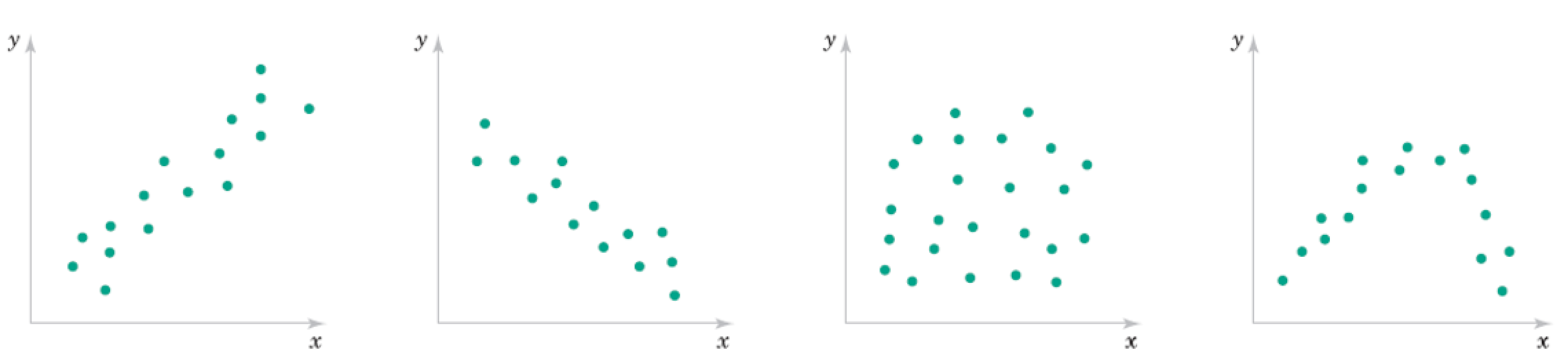
Suppose we know a relationship is quadratic. What can we do?
If we know the relationship is quadratic, we could just take the square root and make it linear.
Old: \begin{align} \mathbf y = \beta_0 + \beta_1 \mathbf x_{(1)} + \beta_2 \mathbf x_{(2)} +...+ \beta_n \mathbf x_{(n)} + \varepsilon , \; \; \; \mathbf x_{(i)} = \begin{bmatrix} x_{(i),1} \\x_{(i),2} \\ \vdots \\ x_{(i),m} \end{bmatrix} \end{align}
New: \begin{align} \mathbf y = \beta_0 + \beta_1 \mathbf x'_{(1)} + \beta_2 \mathbf x'_{(2)} +...+ \beta_n \mathbf x'_{(n)} + \varepsilon, \;\;\; \mathbf x'_{(i)} = \begin{bmatrix} f_{(i)}(x_1) \\f_{(i)}(x_2) \\ \vdots \\ f_{(i)}(x_m) \end{bmatrix} \end{align}
...Feature Engineering, Kernel methods, ...
New model: $\mathbf y = \beta_0 + \beta_1 \mathbf x'_{(1)} + \beta_2 \mathbf x'_{(2)} +...+ \beta_n \mathbf x'_{(n)} + \varepsilon$
$$\mathbf x'_{(i)} = \begin{bmatrix} f_{(i)}(x_1) \\f_{(i)}(x_2) \\ \vdots \\ f_{(i)}(x_m) \end{bmatrix} = \begin{bmatrix} x_{1}^i \\x_{2}^i \\ \vdots \\ x_{m}^i \end{bmatrix}$$Exercise: write the model equations out for 3D case, i.e. $\bf x$ is just $x_1$, $x_2$, and $x_3$.
Use numpy polyfit and polyval to plot the residual versus polynomial order
show_polyfit_ho_example_results(dosage,conc_noisy,(1,2,3,4,5,6));
order: 1, residual: 56.6204627002199
order: 2, residual: 43.28483436298878
order: 3, residual: 38.90189854595423
order: 4, residual: 21.166171682768383
order: 5, residual: 13.416800916508517
order: 6, residual: 1.8203750586044797e-11
