BDS 761: Data Science and Machine Learning I

Topic 5: Regression - 3. Regularization

References

• "An introduction to statistical learning: Python edition", G James, D Witten, T Hastie, R Tibshirani, J Taylor, Springer 2023. https://www.statlearning.com/
• https://developers.google.com/machine-learning/crash-course/linear-regression

Maximum a Posteriori (MAP) Estimation

Again the system: $\mathbf y = \mathbf X \boldsymbol\beta + \boldsymbol\varepsilon$.

Now we seek to maximize the posterior distribution $p(\boldsymbol\beta | \mathbf y; \mathbf X)$ (statisticians also call this maximum likelihood).

The noise is Normally distributed with $\boldsymbol\varepsilon \sim N(\mathbf 0,\sigma_2^2 \mathbf I)$.

Assume the solution has a prior $\boldsymbol\beta \sim N(\mathbf 0,\sigma_1^2 \mathbf I)$

Use Bayes Law to solve for the Posterior distribution $p(\boldsymbol\beta | \mathbf y) = \dfrac{p(\mathbf y |\boldsymbol\beta) p(\boldsymbol\beta)}{p(\mathbf y)}$

Make a simpler optimization problem for finding the maximizer $\boldsymbol\beta^*$ for this. Hint: the denominator does not depend on $\boldsymbol\beta$.

Regression as Optimization

\begin{align} \text{Linear Regression: } \boldsymbol\beta_{lr}^* &= \arg\min\limits_{\boldsymbol\beta} \Vert \mathbf y - \mathbf X \boldsymbol\beta \Vert^2\\ \text{Ridge Regression: } \boldsymbol\beta_{rr}^* &= \arg\min\limits_{\boldsymbol\beta} \Vert \mathbf y - \mathbf X \boldsymbol\beta \Vert^2 + \lambda \Vert \boldsymbol\beta \Vert^2 \end{align}

Note these can be solved analytically with pseudoinverse or SVD techniques (which also provide some diffent kinds of variants).

Recall the $\beta_0$ bias term, how should it have been handled here?

Maximum a Posterior (MAP) Estimation II: "Laplace prior"

Again the system: $\mathbf y = \mathbf X \boldsymbol\beta + \boldsymbol\varepsilon$.

The noise is Normally distributed with $\boldsymbol\varepsilon \sim N(\mathbf 0,\sigma_2^2 \mathbf I)$.

Now the solution has a prior $\boldsymbol\beta \sim C \exp\big( \sum_i^n |\beta_i|\big)$. $C$ is a constant. This is sometimes called a Laplace distribution.

Use Bayes Law to solve for the Posterior distribution.

Make a simpler optimization problem for finding the maximizer $\boldsymbol\beta^*$ for this.

FYI: Full-on Bayesian Inference

While MAP estimation uses Bayes Law, it is not called Bayesian inference.

Maximum Likelihood and MAP estimates are examples of "point estimates".

A Bayesian Inference technique estimates the entire posterior distribution, meaning $\boldsymbol\mu$ and $\boldsymbol\Sigma$ in the prior example.

From this we can estimate many things, such as,

• the mean value of $\boldsymbol\beta$ $\rightarrow$ a (better?) point estimate versus maximum.
• the variance of $\boldsymbol\beta$ $\rightarrow$ confidence intervals.

Take home Messages (updated)

• A $\ell_2$ residual minimization (e.g. norm-squared or variance) implies a Gaussian noise assumption.

• A $\ell_2$ Penalty term implies a Gaussian prior assumption

• A $\ell_1$ Penalty term implies a Laplace prior assumption

• ...where does the regularization parameter come from (exercise)

Regression as Optimization (updated)

\begin{align} \text{Linear Regression: } \boldsymbol\beta_{lr}^* &= \arg\min\limits_{\boldsymbol\beta} \Vert \mathbf y - \mathbf X \boldsymbol\beta \Vert_2^2\\ \text{Ridge Regression: } \boldsymbol\beta_{rr}^* &= \arg\min\limits_{\boldsymbol\beta} \Vert \mathbf y - \mathbf X \boldsymbol\beta \Vert_2^2 + \lambda \Vert \boldsymbol\beta \Vert_2^2 \\ \text{"LASSO": } \boldsymbol\beta_{lasso}^* &= \arg\min\limits_{\boldsymbol\beta} \Vert \mathbf y - \mathbf X \boldsymbol\beta \Vert_2^2 + \lambda \Vert \boldsymbol\beta \Vert_1 \end{align}

Later, Logistic version of everything for Classification.

Lab: Least-squares regression various ways

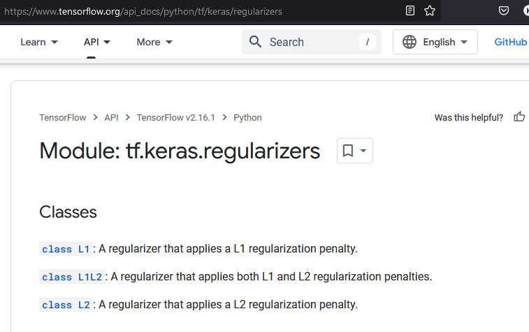
Now compare L1 and L2 regularization in your approach to the previous lab:

Load Boston house prices dataset.

Formulate linear system and try using inverse and pseudoinverse to solve.

Regression: $ \mathbf A \boldsymbol{\beta} \rightarrow \text{target} $

Linear Algebra: solve $ \mathbf A \boldsymbol{\beta} = \text{target} $ for unknown $\boldsymbol{\beta}$.