BDS 761: Data Science and Machine Learning I

Python-based scientific computing package with two primary components/goals:
import numpy as np
import torch
import datetime

print(datetime.datetime.now())
print('torch', torch.__version__)
device = "cuda" if torch.cuda.is_available() else "cpu"
print('device:',device)
2026-09-12 02:46:28.540157
torch 2.10.0+cu128
device: cuda
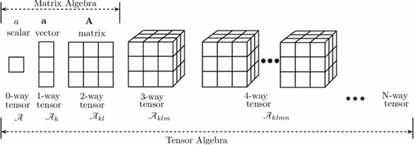
The "tensor dimension" is separate from the dimensionality of each vector space
Tensor dimension also called "tensor rank", not same as rank from linear algebra
Behind the scenes it's just another 1D list of numbers with extra meta info regarding dimensions
Tensor algebra typically uses specialized notation originally by Ricci
Sometimes called Ricci, but in CS commonly called Einstein notation
In physics, Einstein Summation convention (ESC) is a shorthand for sums in index notation
A tensor is written as, e.g., $A_{ijk}$, (which can also mean the $(i,j,k)th$ element of the tensor).
In ESC, repeated indices are meant to be summed over, so $A_{ijk}B_{mnk} = \sum_k A_{ijk}B_{mnk} = C_{ijmn}$
Ai = [1,2,3,4]
Bij = [[1,2,3,4], [5,6,7,8]]
Cijk = [[[1,2,3,4], [5,6,7,8]], [[9,10,11,12], [13,14,15,16]]]
Cijk[1][0][2] # what are i,j,k here?
11
from sklearn.datasets import load_sample_images

dat = load_sample_images()
print(dat.keys(), dat['filenames'])
img = dat['images'][0]
print(img.shape)
dict_keys(['images', 'filenames', 'DESCR']) ['china.jpg', 'flower.jpg']
(427, 640, 3)
from matplotlib.pyplot import *
imshow(img);

https://docs.scipy.org/doc/numpy-1.13.0/reference/arrays.ndarray.html
A $d$-dimensional data structure, containing $n_1\times n_2 \times ... \times n_d$ numbers
import numpy as np
type(np.array([1,2,3]))
numpy.ndarray
import numpy as np

np.random.rand(3)
array([0.27675517, 0.41849231, 0.58769562])
np.random.rand(3,2) # note not a tuple (unlike many other numpy functions)
array([[0.67056542, 0.12513284],
       [0.32786265, 0.59226601],
       [0.98372305, 0.38512455]])
np.random.rand(3,2,4)
array([[[0.84073156, 0.94746165, 0.52019364, 0.48644409],
        [0.2211287 , 0.71658406, 0.84742256, 0.78154493]],

       [[0.6154219 , 0.09136686, 0.08475093, 0.24412863],
        [0.95182114, 0.49359319, 0.57891852, 0.21951896]],

       [[0.76570532, 0.68853465, 0.59700395, 0.29172765],
        [0.80931308, 0.03689716, 0.46926175, 0.86785482]]])
T = np.random.rand(3,2,4,3,2)
T.shape, T.ndim
((3, 2, 4, 3, 2), 5)
Very similar to NumPy’s ndarray. But with lots of support for doing things efficiently (manually).
A = torch.tensor([1, 2, 3])
print(A)
tensor([1, 2, 3])
Note uninitialized matrix contains whatever values were in the allocated memory at the time
x = torch.empty(3, 4)
print(x)
tensor([[-4.6675e+07,  4.2396e-41,  2.3591e-24,  3.3927e-41],
        [ 4.4842e-44,  0.0000e+00,  1.1210e-43,  0.0000e+00],
        [-8.3627e+29,  3.3931e-41,  0.0000e+00,  0.0000e+00]])
x = torch.zeros(3, 4, dtype=torch.long) # "initialized" tensor
print(x)
A = torch.rand(3, 5)
print(A)
tensor([[0.4358, 0.3858, 0.2403, 0.8578],
        [0.2246, 0.3507, 0.5784, 0.6390],
        [0.5340, 0.6322, 0.4748, 0.1581]])
Reuse some of previous meta information, depending on inputs (such as same dtype, or shape)
x = x.new_ones(5, 3, dtype=torch.double) # change shape, also dtype possible
print(x)
tensor([[1., 1., 1.],
        [1., 1., 1.],
        [1., 1., 1.],
        [1., 1., 1.],
        [1., 1., 1.]], dtype=torch.float64)
x = torch.randn_like(x, dtype=torch.float)    # replace dtype
print(x)                                      # result has the same size
tensor([[-1.7514, -0.8170, -0.8062],
        [ 0.3534, -1.7679, -1.0424],
        [ 1.2540, -0.7745, -1.2885],
        [ 0.5158,  1.5432,  1.0822],
        [-0.1090,  1.5805, -1.3659]])
print(x.size())
print(x.shape)
torch.Size([3, 4])
torch.Size([3, 4])
x = torch.rand(5, 3)
print(x)
print('')
print(x[:, 1])
tensor([[0.8749, 0.2819, 0.8611],
        [0.7026, 0.8043, 0.6709],
        [0.1154, 0.9857, 0.5036],
        [0.1527, 0.9233, 0.9340],
        [0.0364, 0.2090, 0.2790]])

tensor([0.2819, 0.8043, 0.9857, 0.9233, 0.2090])
print(x[1,:])
tensor([-1.1725, -1.7245, 1.3550])
print(x[1,[True, False, True]])
tensor([-1.1725, 1.3550])
x[0,0]
tensor(-0.1049)
x[0,0].item()
-0.10485438257455826
Note that this is a reference to the tensor, not a copy
y = x.numpy()
print(y)
[[-0.10485438  1.2708315  -1.4843239  -1.8760405 ]
 [-0.45950317 -1.0605842   0.32289705 -1.1333894 ]
 [-0.7912421   0.5949042   0.25584257  0.7625179 ]
 [-0.38327378  0.26073715  0.87647516  1.4194298 ]]
x.add_(10) # in-place add
print(x)
print(y)
tensor([[19.8951, 21.2708, 18.5157, 18.1240],
        [19.5405, 18.9394, 20.3229, 18.8666],
        [19.2088, 20.5949, 20.2558, 20.7625],
        [19.6167, 20.2607, 20.8765, 21.4194]])
[[19.895145 21.270832 18.515676 18.123959]
 [19.540497 18.939415 20.322897 18.866611]
 [19.208757 20.594904 20.255842 20.762518]
 [19.616726 20.260738 20.876476 21.41943 ]]
import numpy as np
a = np.ones(5)
b = torch.from_numpy(a)
np.add(a, 1, out=a)
print(a)
print(b)
[2. 2. 2. 2. 2.]
tensor([2., 2., 2., 2., 2.], dtype=torch.float64)
Multiple syntaxes for the same operations
Note: trailing underscore means in-place operation for tensor, .copy(), .t()
x = torch.rand(3, 2)
y = torch.rand(3, 2)

print(x,'\n')
print(y,'\n')

print(x + y)
tensor([[0.3522, 0.9329],
        [0.8709, 0.8470],
        [0.8909, 0.6978]])

tensor([[0.0676, 0.0066],
        [0.2154, 0.4033],
        [0.8985, 0.8056]])

tensor([[0.4198, 0.9394],
        [1.0863, 1.2503],
        [1.7894, 1.5034]])
print(torch.add(x, y))
tensor([[0.4198, 0.9394],
        [1.0863, 1.2503],
        [1.7894, 1.5034]])
result = torch.empty(3, 2)
torch.add(x, y, out=result)
print(result)
tensor([[0.4198, 0.9394],
        [1.0863, 1.2503],
        [1.7894, 1.5034]])
print(x + y,'\n')

y.add_(x) # in-place version
print(y)
tensor([[0.4198, 0.9394],
        [1.0863, 1.2503],
        [1.7894, 1.5034]])

tensor([[0.4198, 0.9394],
        [1.0863, 1.2503],
        [1.7894, 1.5034]])
For efficiency, you are given low-level control of the storage, including
GPU as a specialized assistant "co-processor" - The CPU (host) runs the program and handles high-level decisions, then hands off intensive processing tasks to the GPU as needed.
In C this can be controlled in detail manually.
In python we move the data (the tensor) and the function gets run on the device based on where the data is located.
Can move to any GPU you have, e.g. CUDA:0, CUDA:1, ...
Many packages such as CuPy do memory transfers for you.
import torch
device = torch.device("cuda:0" if torch.cuda.is_available() else "cpu") # cuda:0 = 1st gpu
print(device)
cuda
x = torch.ones((3, 3), device=device)
print(x)
tensor([[1., 1., 1.],
        [1., 1., 1.],
        [1., 1., 1.]], device='cuda:0')
change device or data type
y_cpu = torch.zeros(5, device='cpu')
print(y_cpu)
print(y_cpu.type(),'\n')

# Transfer from CPU memory to device memory
y_device = y_cpu.to(device)
print(y_device)

print(y_device.type())
tensor([0., 0., 0., 0., 0.])
torch.FloatTensor

tensor([0., 0., 0., 0., 0.], device='cuda:0')
torch.cuda.FloatTensor
y_float = y_cpu.to(torch.float32)
print(y_float)
tensor([0., 0., 0., 0., 0.])
torch.set_default_device("cuda:0")

# Automatically allocated on cuda:0 without explicit device arguments
z = torch.randn(2, 2)
print(z)
tensor([[-0.2638, -1.3707],
        [ 0.7307,  0.4409]], device='cuda:0')
Overwhelmingly, the "tensors" everyone uses are processed as matrix and vectors, i.e. linear algebra packages you know.
Behind the scenes the data is always a 1D list of numbers with some meta-info regarding dimensions
We just need a few new tricks.
(There is actual higher-order versions of linear algebra, referred to as Tensor operations, such as Tucker decompositions, but this is a small and specialized research topic.)
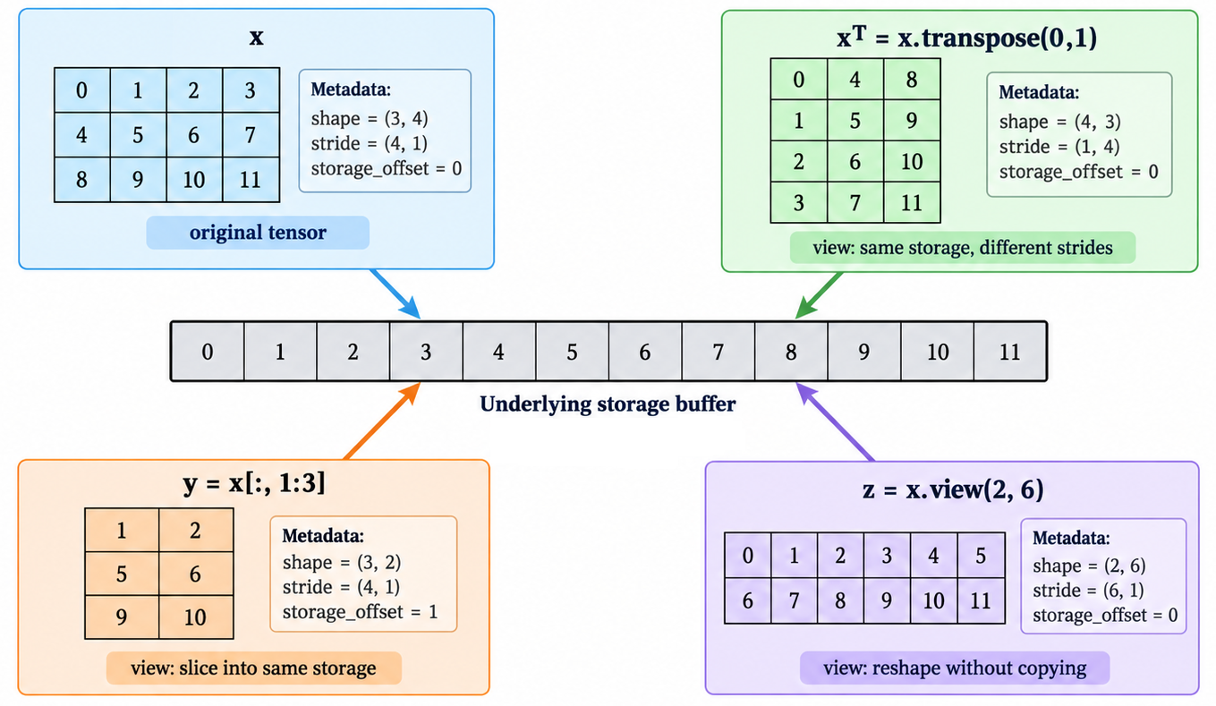
The underlying memory buffer is managed by a Storage instance, representing a one-dimensional, contiguous array of typed memory.
Tensors function as views into a Storage object, defined by metadata attributes: size (shape), stride, and storage offset.
Multiple tensors can reference the same storage instance. Operations involving slicing, reshaping, or axis permutation modify the metadata attributes without reallocation or copying of the underlying memory.
import torch

A = torch.tensor([[1.0, 2.0], [3.0, 4.0]])

storage = A.untyped_storage() # Access the underlying memory buffer

storage.data_ptr()
103985859345728
A = torch.arange(12) # 1D array
B = A.view(3,4)
print(B)
tensor([[ 0,  1,  2,  3],
        [ 4,  5,  6,  7],
        [ 8,  9, 10, 11]])
Transpose as swapping rows and cols --> index $0 \leftrightarrow 1$, presuming fixed meaning of indices: row, column, ...?
More generally, for $n$-dimensional tensor, give the pair of tensors to transpose across
A = torch.tensor([[1.0, 2.0], [3.0, 4.0]])
B = A.transpose(0, 1)

B[0, 1] = 99.0

print(A)
print(B)
tensor([[ 1.,  2.],
        [99.,  4.]])
tensor([[ 1., 99.],
        [ 2.,  4.]])
compare the data_ptr for these
All data is stored in 1D arrays behind the scenes. Meta info gives its shape.
The mapping from 1D to that shape is called the layout
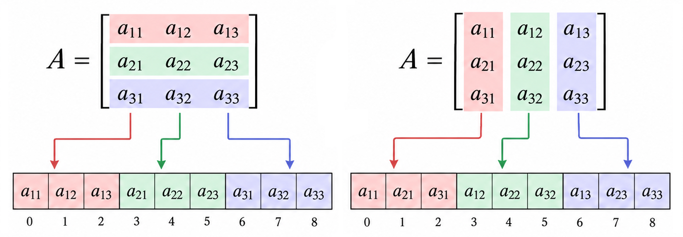
What element in the 1D array contains $A_{ij}$ for each storage format? Make a formula $k = f(i,j)$
Consider a matrix stored in an array in memory. How do you get the array location $k$ for the matrix element $i,j$?
help(x.stride)
Help on built-in function stride:

stride(...) method of torch.Tensor instance
    stride(dim) -> tuple or int

    Returns the stride of :attr:`self` tensor.

    Stride is the jump necessary to go from one element to the next one in the
    specified dimension :attr:`dim`. A tuple of all strides is returned when no
    argument is passed in. Otherwise, an integer value is returned as the stride in
    the particular dimension :attr:`dim`.

    Args:
        dim (int, optional): the desired dimension in which stride is required

    Example::

        >>> x = torch.tensor([[1, 2, 3, 4, 5], [6, 7, 8, 9, 10]])
        >>> x.stride()
        (5, 1)
        >>> x.stride(0)
        5
        >>> x.stride(-1)
        1
x = torch.arange(3*4).view(3,4)
print(x)
tensor([[ 0,  1,  2,  3],
        [ 4,  5,  6,  7],
        [ 8,  9, 10, 11]])
print(x.stride())
(4, 1)
x = torch.arange(3*4*5).view(3,4,5)

x.stride()
(20, 5, 1)
Operations to convert matrices into vectors and vice-versa
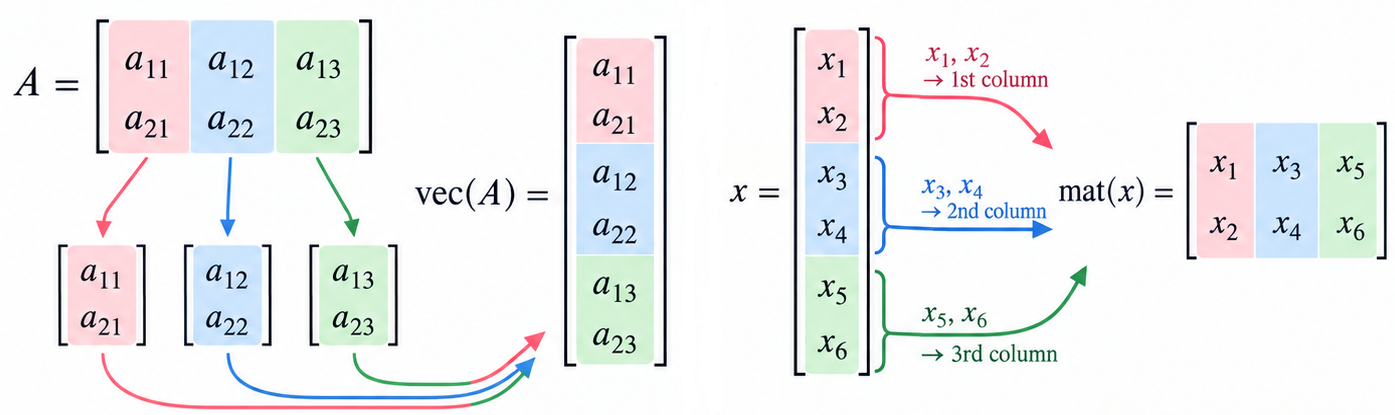
The can actually be implemented with tensor multiplication, but it's obvious enough how to do it directly.
Note: in software, converting scalar operation into array operation as with numpy is also called "vectorization".
The Kronecker product as a way to perform the tensor product while staying in matrix shape.
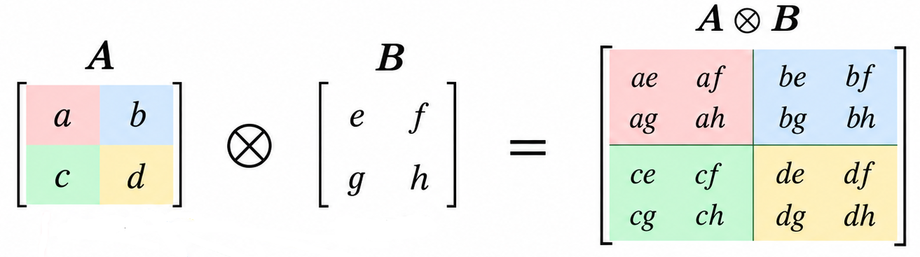
Treat vectors and scalars as special cases of matrices
Converts a product of matrices into a matrix-vector product:
$$\operatorname{vec}(ABC) = (C^T \otimes A) \operatorname{vec}(B)$$import numpy as np
A = np.eye(2)
B = np.array([[1, 2], [3, 4]])
C = np.array([[1], [-1]])
# 'F' specifies Fortran-like index order = column-major vectorization
vec_ABC = (A @ B @ C).flatten('F')
np.kron(C.T, A) @ B.flatten('F')
array([-1., -1.])
Give the matrix system $AXB = C$, use the kronecker product identity to solve for unknown $X$ in terms of matrices $A$, $B$, and $C$.
Why is this important when it only involves vectors and matrices?
Answer: because we can break down almost all tensor operations we do in modern AI into matrix operations, then convert into matrix-vector operations to utilize our linear algebra tools.
Just change the meta info to change the mapping used for different shapes, generally with same total number of elements.
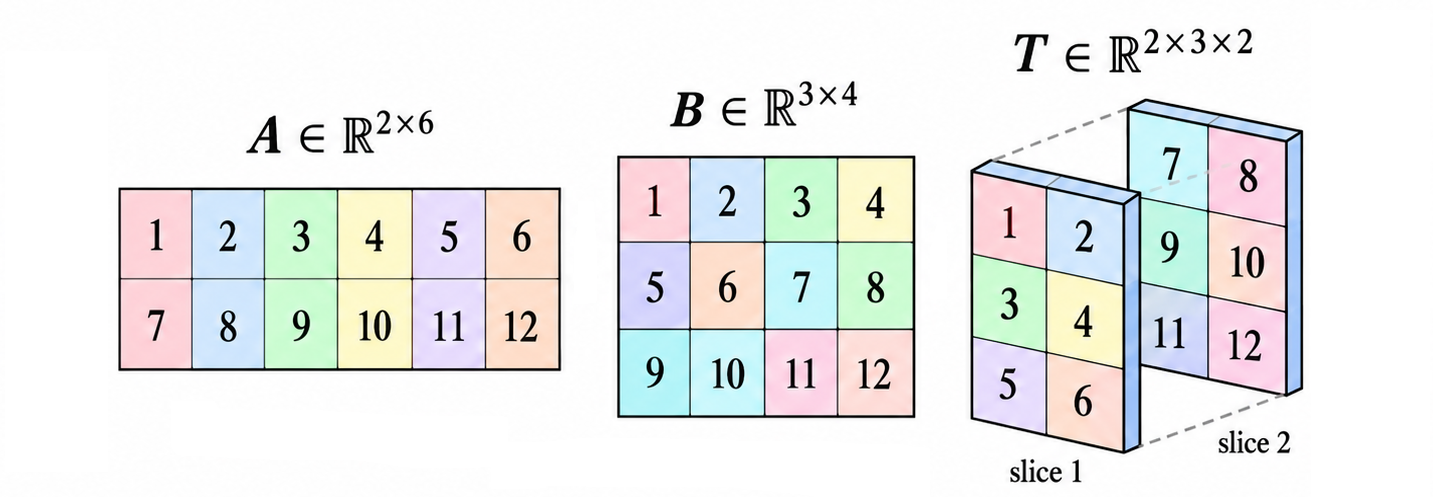
Think of as a generalization of the vectorization and matricization, along with related operations like transpose
Like vectorize, but instead of getting $N \times 1$ ndarray, get "flat" array size="$(N,0)$"
Think of as "just give me the numbers"
matlab "A(:)"
import numpy as np

np.ndarray.flatten?
A = np.array([[1,2],[3,4]])
print(A)
print('')
print(A.flatten('C')) # "C style" -> treat as list of rows
print('')
print(A.flatten())
[[1 2]
 [3 4]]

[1 2 3 4]

[1 2 3 4]
A = np.array([[1,2],[3,4]])
print(A)
print('')
print(A.flatten('F')) # "Fortran style" -> treat as list of cols
[[1 2]
 [3 4]]

[1 3 2 4]
Cijk = np.array([[[1,2,3,4], [5,6,7,8]], [[9,10,11,12],[13,14,15,16]],[[17,18,19,20],[21,22,23,24]]])

Cijk.shape
(3, 2, 4)
Cijk.flatten().shape
(24,)
Cijk.flatten()
array([ 1,  2,  3,  4,  5,  6,  7,  8,  9, 10, 11, 12, 13, 14, 15, 16, 17,
       18, 19, 20, 21, 22, 23, 24])
A.flatten or torch.flatten(A)
Takes args allowing range of dims to flatten.
Always row-major format assumed.
x = torch.randn(2,2,2)
print(x, '\n')
print(x.flatten())
tensor([[[-1.4625, -0.3584],
         [-1.4370, -0.2888]],

        [[ 0.0028, -0.1341],
         [ 0.7152,  0.1152]]])

tensor([-1.4625, -0.3584, -1.4370, -0.2888,  0.0028, -0.1341,  0.7152,  0.1152])
x.flatten(start_dim=1, end_dim=-1)
tensor([[-1.4625, -0.3584, -1.4370, -0.2888],
        [ 0.0028, -0.1341,  0.7152,  0.1152]])
Tries to return a flat view
A = np.array([[1,2],[3,4]])
print(A)
print('')
print(A.ravel('F'))
[[1 2]
 [3 4]]

[1 3 2 4]
A = np.array([[1,2],[3,4]])

b_flat = A.flatten()
b_ravel = A.ravel()

sum(b_flat-b_ravel)
np.int64(0)
b_flat[0] = 999

print(A, b_flat)
[[1 2]
 [3 4]] [999   2   3   4]
b_ravel[0] = 999

print(A, b_ravel)
[[999   2]
 [  3   4]] [999   2   3   4]
A = np.array([[1,2],[3,4]])
print(A)
print(A.shape)
print('')
B = A.reshape(1,4)
print(B,B.shape)
[[1 2]
 [3 4]]
(2, 2)

[[1 2 3 4]] (1, 4)
x = torch.randn(4, 4)
y = x.view(16)
print(y)
print(x.size(), y.size())
tensor([-0.1049,  1.2708, -1.4843, -1.8760, -0.4595, -1.0606,  0.3229, -1.1334,
        -0.7912,  0.5949,  0.2558,  0.7625, -0.3833,  0.2607,  0.8765,  1.4194])
torch.Size([4, 4]) torch.Size([16])
z = x.view(-1, 8)  # the size -1 is inferred from other dimensions
print(x.size(), z.size())
torch.Size([4, 4]) torch.Size([2, 8])
x = torch.arange(6)
y = x.view(2, 3)
print(x)
print(y)
tensor([0, 1, 2, 3, 4, 5])
tensor([[0, 1, 2],
        [3, 4, 5]])
y[0,2] = 999
print(x)
print(y)
tensor([  0,   1, 999,   3,   4,   5])
tensor([[  0,   1, 999],
        [  3,   4,   5]])
x = torch.arange(6).reshape(2,3)
y = x.transpose(0, 1)
print(x)
print(y)
tensor([[0, 1, 2],
        [3, 4, 5]])
tensor([[0, 3],
        [1, 4],
        [2, 5]])
y[0,1] = 999
print(x)
print(y)
tensor([[  0,   1,   2],
        [999,   4,   5]])
tensor([[  0, 999],
        [  1,   4],
        [  2,   5]])
Transpose as permuting rows and cols $\rightarrow$ dims [0,1] permuted to [1,0]
np.permute_dims?
A = np.array([[1,2],[3,4]])
print(A)
print('')
print(np.permute_dims(A,[1,0]))
[[1 2]
 [3 4]]

[[1 3]
 [2 4]]
Cijk = np.array([[[1,2,3,4], [5,6,7,8]], [[9,10,11,12],[13,14,15,16]],[[17,18,19,20],[21,22,23,24]]])

print(Cijk.shape)

print(np.permute_dims(Cijk,[0,2,1]).shape)
(3, 2, 4)
(3, 4, 2)
Allows reordering all tensor dims, not just two
also modifies strides and returns a view.
w = torch.zeros(2, 3, 4)
print(w.shape)
v = w.permute(2, 0, 1)
print(v.shape)
torch.Size([2, 3, 4])
torch.Size([4, 2, 3])
A vision transformer is an approach to apply the attention mechanism to images, creating models which can be made vastly larger and trained on more data.
Variations are used as the image "encoding" component for most VLMs (vision language models).

As teh title indicates, the vision transformer divides the image into $16 \times 16 \times 3$ color pixel blocks, and treating these analogous to speech tokens.
E.g. instead of a vector representing the word 'the' it is a vector representing a small color patch image of an eye.
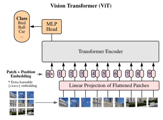
A vision transformer is a basic approach to apply the attention mechanism to images by chopping the image into $16 \times 16 \times 3$ color pixel blocks, and treating these as length-768 vectors analogous to speech tokens.
E.g. instead of a vector representing the word 'the' it is a vector representing a small color patch image of an eye.
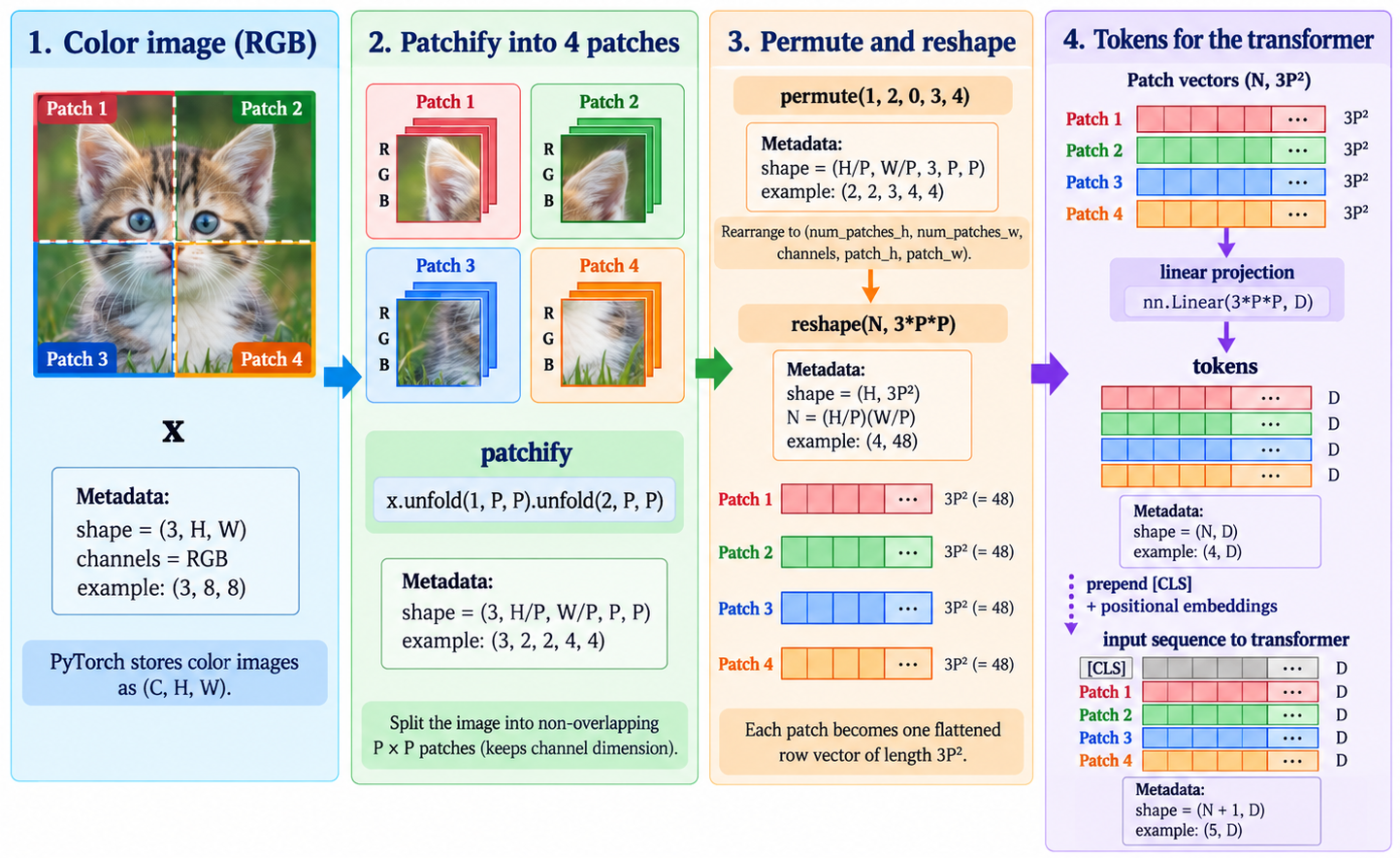
Let $X \in \mathbb{R}^{B \times C \times H \times W}$ represent a batch of images
Let $P$ denote the patch resolution (e.g., 16)
import torch

B, C, H, W, P = 2, 3, 224, 224, 16
x = torch.randn(B, C, H, W) # a test batch of images
print(x.shape)
torch.Size([2, 3, 224, 224])
Think in terms of list of lists perspective:
The outermost index is $B$, so $x$ is a list (i.e., batch) of images
Next is $C$, so there's a separate image for each color, in a list of 3.
Last is a list of $H$ rows, each of length $W$
Decompose spatial dimensions $H$ and $W$ into a patch grid, yielding $X_{\text{grid}} \in \mathbb{R}^{B \times C \times \frac{H}{P} \times P \times \frac{W}{P} \times P}$. This partitions the C-contiguous memory layout without reallocation.
x_grid = x.view(B, C, H // P, P, W // P, P) # // means integer division, so truncating result to integer
print(x_grid.shape)
torch.Size([2, 3, 14, 16, 14, 16])
Isolate the patch grid coordinates from the intra-patch pixel coordinates, yielding $X_{\text{perm}} \in \mathbb{R}^{B \times \frac{H}{P} \times \frac{W}{P} \times C \times P \times P}$.
x_perm = x_grid.permute(0, 2, 4, 1, 3, 5)
print(x_perm.shape)
torch.Size([2, 14, 14, 3, 16, 16])
Flatten the 2 dims representing row versus col location of patch into a single dim of length $N = \frac{H \cdot W}{P^2}$
flatten innermost list of lists of lists, describing color patches into vectors of dimension $D_{\text{patch}} = C \cdot P^2$, yielding $X_{\text{flat}} \in \mathbb{R}^{B \times N \times D_{\text{patch}}}$.
Because the prior permutation destroys contiguity, this reshape requires memory reallocation to achieve desired shape (equivalent to .contiguous().view()).
N = (H // P) * (W // P)
D_patch = C * P * P
x_flat = x_perm.reshape(B, N, D_patch)
print(x_flat.shape)
torch.Size([2, 196, 768])
So the result is a batch of 196 vectors, each of which represents a patch of the image.
from nbtools01 import *
printcols(dir(torch.linalg))
LinAlgError          _linalg              eigvalsh             lu_solve             solve
__builtins__         cholesky             householder_product  matmul               solve_ex
__cached__           cholesky_ex          inv                  matrix_exp           solve_triangular
__doc__              common_notes         inv_ex               matrix_norm          svd
__file__             cond                 ldl_factor           matrix_power         svdvals
__loader__           cross                ldl_factor_ex        matrix_rank          tensorinv
__name__             det                  ldl_solve            multi_dot            tensorsolve
__package__          diagonal             lstsq                norm                 vander
__path__             eig                  lu                   pinv                 vecdot
__spec__             eigh                 lu_factor            qr                   vector_norm
_add_docstr          eigvals              lu_factor_ex         slogdet
X_centered = X - X.mean(dim=0)
covariance_matrix = (X_centered.T @ X_centered) / (X.shape[0] - 1)

U, S, V = torch.linalg.svd(covariance_matrix)
principal_components = U[:, :2]
X_reduced = X_centered @ principal_components
For the breast cancer dataset, select a random batch of 8 subjects. For each , find the indices of the $k$ most similar patients. Do not use loops.
torch.cdist - Compute the batched $p$-norm distance between each pair of the two collections of row vectors.
torch.topk - Returns the $k$ largest elements of the given input tensor along a given dimension.
https://docs.pytorch.org/docs/2.14/generated/torch.cdist.html
https://docs.pytorch.org/docs/2.14/generated/torch.topk.html