BDS 761: Data Science and Machine Learning I

People are now making billions of dollars using derivatives from High School calculus. And not the really tricky ones.
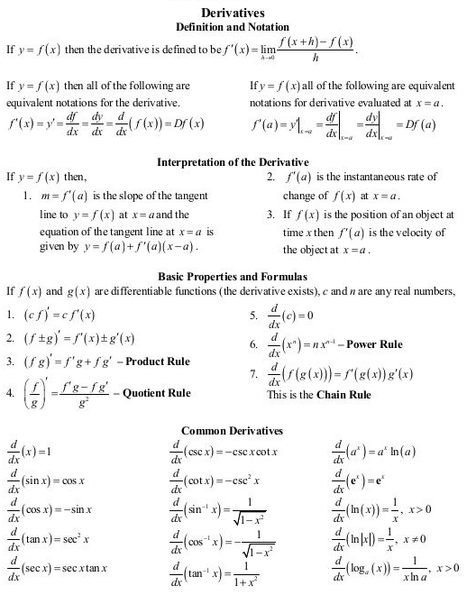
If $y=f(x)$, the derivative is defined by
$$ f'(x)=\lim_{h\to0}\frac{f(x+h)-f(x)}{h}. $$Equivalent notations:
$$ f'(x)=y'=\frac{df}{dx}=\frac{dy}{dx} =\frac{d}{dx}\bigl(f(x)\bigr)=Df(x). $$Evaluated at $x=a$:
$$ f'(a) =\left.y'\right|_{x=a} =\left.\frac{df}{dx}\right|_{x=a} =\left.\frac{dy}{dx}\right|_{x=a} =Df(a). $$$f'(a)$ is the slope of the tangent line to $y=f(x)$ at $x=a$. The tangent line is $$ y=f(a)+f'(a)(x-a). $$
Or $f'(a)$ is the instantaneous rate of change of $f$ at $x=a$.
If $f(t)$ describes position at time $t$, and $f'(a)$ is velocity at $t=a$.
A polynomial in $x$ with terms scaled by the derivatives (and a factorial).
\begin{align} f(x) &= \sum_{k=0}^n \frac{1}{k!} \left.\frac{d^k f(x)}{dx^k} \right|_a (x-a)^k \notag\\ &= f(a) + f'(a)(x-a) + \frac{1}{2}f''(a)(x-a)^2 + ... \notag \end{align}This is the first-order Taylor expansion of $f$ at $a$, which can be used as a local approximation.
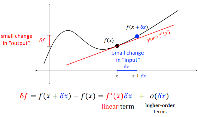
What does this say in physics terms when $f(t)$ describes position at time $t$, and $f'(a)$ is velocity at $t=a$?
Generally what is a local linear approximation of a function useful for?
Finding max or min by setting derivative equal to zero
Gradient descent for minimizing function
Find location and value of minimum of $J(w) = w^2 - 2w + 5$.
Solve this using gradient descent manually starting from $w=0$
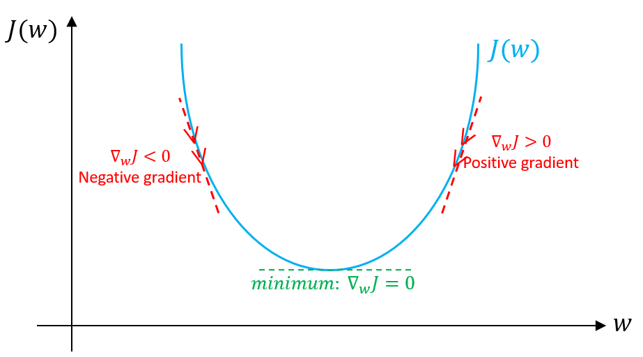
"$J$" denotes the objective function, meaning the thing optimized. We pick what $J$ is based on our goal.
figure(figsize=(4,2))
z = np.arange(-10, 10, 0.1)
plot(z, 1 / (1 + np.exp(-z)), linewidth=3);
xlabel('z');
ylabel('sigma(z)');

Scavenger Hunt: Find the derivative of the sigmoid($z$) wrt $z$
The activation function that was popular when Deep Learning became famous.
figure(figsize=(4,2))
z = np.arange(-10, 10, 0.1)
plot(z, [max(0, i) for i in z], linewidth=3);
xlabel('z');
ylabel('ReLU(z)');

What is its derivative?
For a convex function $f$, a vector $g$ is a subgradient at point $x_0$ if it satisfies the following for all $x$ $$ f(x) \geq f(x_0) + g^T(x - x_0) $$ Note the linear approximation created by the subgradient $g$ always sits completely on or below the actual function.
$\partial f(x_0)$ is the set of all valid subgradients at $x_0$, called the subdifferential.
At the non-differentiable point $x = 0$, the slopes on either side are $\alpha$ and $1$.
Therefore, the subdifferential is the closed interval $\partial f(0) = [\alpha, 1]$.
In practice, we can just pick anything from that set to use as the derivative, say assume it is zero. It will work in the local approximation perspective for optimization.
(recall this is all usually operating in finite precision also)
Exercise: Absolute value - What is the gradient and/or subgradient that you would use for $|x|$
Assume $f$ and $g$ are differentiable and $c,n$ are constants. Rules apply wherever the expressions are defined and differentiable.
| ............Rule........... | ..............Formula............................ |
|---|---|
| Constant scalar | $\displaystyle (cf)'=cf'$ |
| Sum and difference | $\displaystyle (f\pm g)'=f'\pm g'$ |
| Product | $\displaystyle (fg)'=f'g+fg'$ |
| Quotient | $\displaystyle \left(\frac{f}{g}\right)'=\frac{f'g-fg'}{g^2},\quad g\ne0$ |
| Constant | $\displaystyle \frac{d}{dx}(c)=0$ |
| Power | $\displaystyle \frac{d}{dx}(x^n)=nx^{n-1}$ |
| Chain | $\displaystyle \frac{d}{dx}f(g(x))=f'(g(x))\,g'(x)$ |
Identity and Trigonometric Functions
$$ \begin{aligned} \frac{d}{dx}(x) &= 1 \\[6pt] \frac{d}{dx}(\sin x) &= \cos x \\[6pt] \frac{d}{dx}(\cos x) &= -\sin x \\[6pt] \frac{d}{dx}(\tan x) &= \sec^2 x \\[6pt] \frac{d}{dx}(\cot x) &= -\csc^2 x \\[6pt] \frac{d}{dx}(\sec x) &= \sec x\tan x \\[6pt] \frac{d}{dx}(\csc x) &= -\csc x\cot x \end{aligned} $$Inverse Trigonometric Functions
$$ \begin{aligned} \frac{d}{dx}(\arcsin x) &= \frac{1}{\sqrt{1-x^2}}, && |x|<1 \\[8pt] \frac{d}{dx}(\arccos x) &= -\frac{1}{\sqrt{1-x^2}}, && |x|<1 \\[8pt] \frac{d}{dx}(\arctan x) &= \frac{1}{1+x^2}, && x\in\mathbb{R} \end{aligned} $$Exponential and Logarithmic Functions
$$ \begin{aligned} \frac{d}{dx}(a^x) &= a^x\ln a, && a>0 \\[8pt] \frac{d}{dx}(e^x) &= e^x \\[8pt] \frac{d}{dx}(\ln x) &= \frac{1}{x}, && x>0 \\[8pt] \frac{d}{dx}(\ln|x|) &= \frac{1}{x}, && x\ne0 \\[8pt] \frac{d}{dx}(\log_a x) &= \frac{1}{x\ln a}, && x>0,\ a>0,\ a\ne1 \end{aligned} $$Centered version
$$ f'(x) \approx \frac{f(x - \frac{h}{2})-f(x + \frac{h}{2})}{h} \text{ for small number $h$} $$def f(x):
return x**2 + 2*x
def fd_derivative(f, z, eps=0.000001):
return (f(z + eps) - f(z - eps))/(2 * eps)
df_dx = fd_derivative(f, 3, 0.00001)
print(df_dx)
8.00000000005241
from matplotlib.pyplot import *
import numpy as np

def step(z):
    return (z > 0).astype(float)

def sigmoid(z):
    return 1 / (1 + np.exp(-z))

def relu(z):
    return np.maximum(0, z)
z = np.linspace(-5, 5, 200)
figure(figsize=(9,4))
subplot(121)
plot(z, step(z), "r-", linewidth=1, label="Step")
plot(z, sigmoid(z), "g--", linewidth=2, label="Sigmoid")
plot(z, relu(z), "m-", linewidth=2, label="ReLU")
grid()
legend(loc="center right", fontsize=14)
title("Activation functions", fontsize=14)
axis([-5, 5, -.2, 1.2])

subplot(122)
plot(z, fd_derivative(step, z), "r-", linewidth=1, label="Step")
plot(z, fd_derivative(sigmoid, z), "g--", linewidth=2, label="Sigmoid")
plot(z, fd_derivative(relu, z), "m-", linewidth=2, label="ReLU")
grid()
title("FD Derivatives", fontsize=14)
axis([-5, 5, -0.2, 1.2]);

A dual number is an algebraic structure written as $\bar{x} = a + b\epsilon$, where $a$ and $b$ are real numbers and $\epsilon$ is a small non-zero element such that $\epsilon^2 = 0$.
Taylor expansion of $f(\bar{x}) = f(a + b\epsilon)$ about $a$ (the full exact expansion) \begin{align} f(a + b\epsilon) &= f(a) + f'(a)b\epsilon + (\text{infinite higher-order terms}) \times\epsilon^2 \notag \\ &= a' + b'\epsilon + 0 \times \epsilon^2 \notag \end{align}
So we get a dual number with the dual part being $f'(a)$
Dual numbers have their own arithmetic rules, which are generally quite natural. For example:
Addition: $(a_1 + b_1\epsilon) + (a_2 + b_2\epsilon) = (a_1 + a_2) + (b_1 + b_2)\epsilon$
Subtraction: $(a_1 + b_1\epsilon) - (a_2 + b_2\epsilon) = (a_1 - a_2) + (b_1 - b_2)\epsilon$
Multiplication: $(a_1 + b_1\epsilon) \times (a_2 + b_2\epsilon) = (a_1 a_2) + (a_1 b_2 + a_2 b_1)\epsilon + b_1 b_2\epsilon^2 = (a_1 a_2) + (a_1b_2 + a_2b_1)\epsilon$
Division: $\dfrac{a_1 + b_1\epsilon}{a_2 + b_2\epsilon} = \dfrac{a_1 + b_1\epsilon}{a_2 + b_2\epsilon} \cdot \dfrac{a_2 - b_2\epsilon}{a_2 - b_2\epsilon} = \dfrac{a_1 a_2 + (b_1 a_2 - a_1 b_2)\epsilon - b_1 b_2\epsilon^2}{{a_2}^2 + (a_2 b_2 - a_2 b_2)\epsilon - {b_2}^2\epsilon} = \dfrac{a_1}{a_2} + \dfrac{a_1 b_2 - b_1 a_2}{{a_2}^2}\epsilon$
Power: $(a + b\epsilon)^n = a^n + (n a^{n-1}b)\epsilon$
etc.
The use of dual numbers for gradients is called forward-mode automatic differentiation
Must overload operators and functions to handle them, e.g. "+" must add the dual parts appropriately. Similar to array programming or comlpex number handling.
class DualNumber(object):
    def __init__(self, value=0.0, eps=0.0):
        self.value = value
        self.eps = eps
    def __add__(self, b):
        return DualNumber(self.value + self.to_dual(b).value,
                          self.eps + self.to_dual(b).eps)
    def __radd__(self, a):
        return self.to_dual(a).__add__(self)
    def __mul__(self, b):
        return DualNumber(self.value * self.to_dual(b).value,
                          self.eps * self.to_dual(b).value + self.value * self.to_dual(b).eps)
    def __rmul__(self, a):
        return self.to_dual(a).__mul__(self)
    def __str__(self):
        if self.eps:
            return "{:.1f} + {:.1f}ε".format(self.value, self.eps)
        else:
            return "{:.1f}".format(self.value)
    def __repr__(self):
        return str(self)
    @classmethod
    def to_dual(cls, n):
        if hasattr(n, "value"):
            return n
        else:
            return cls(n)
$3 + (3 + 4 \epsilon) = 6 + 4\epsilon$
3 + DualNumber(3, 4)
6.0 + 4.0ε
$(3 + 4ε)\times(5 + 7ε)$ = $3 \times 5 + 3 \times 7ε + 4ε \times 5 + 4ε \times 7ε$ = $15 + 21ε + 20ε + 28ε^2$ = $15 + 41ε + 28 \times 0$ = $15 + 41ε$
DualNumber(3, 4) * DualNumber(5, 7)
15.0 + 41.0ε
x = DualNumber(3.0, 1.0)

def f(x):
    return x*x + 2*x

f(x)
15.0 + 8.0ε
What are the benefits and drawbacks of Dual numbers versus finite-difference derivatives?
Instead of replacing the numbers, we can extend the functions (say as classes in Python) to include their own derivative functions
class Mypow:
    def evaluate(self, x, power):
        return x ** power
    def derivative(self, x, power):
        return power * x ** (power - 1)
    def __call__(self, x, power): # Mypow()(x, power) -> Mypow().evaluate(x, power)
        return self.evaluate(x, power)

def diff(f, args):
    return f.derivative(**args)

Mypow()(3, 2), diff(Mypow(), {'x': 3, 'power': 2})
(9, 6)
Functions for symbolic calculus, equation solving, etc.
Quite handy for dealing with complicated equations
from sympy import *
init_printing(use_unicode=False)

diff(exp(x**2), x)
x = Symbol('x')
integrate(x**2 + x + 1, x)
limit(sin(x)/x, x, 0)
taylor_series = series(cos(x), x, 0, 12)
print("Taylor series of cos(x):", taylor_series)
Taylor series of cos(x): 1 - x**2/2 + x**4/24 - x**6/720 + x**8/40320 - x**10/3628800 + O(x**12)
from sympy import *
x = Symbol('x')

def sigmoid(z):
    return 1 / (1 + exp(-z))

diff(sigmoid(x), x)
diff(sigmoid(x), x).subs(x, 0) # substitute value and simplify
from sympy import *

def step(z):
    return sign(z)

diff(step(x), x)
def relu(z):
    return max(0, z)

diff(relu(x), x)
---------------------------------------------------------------------------
TypeError                                 Traceback (most recent call last)
Cell In[52], line 4
      1 def relu(z):
      2     return max(0, z)
----> 4 diff(relu(x), x)

Cell In[52], line 2, in relu(z)
      1 def relu(z):
----> 2     return max(0, z)

File /usr/local/lib/python3.10/dist-packages/sympy/core/relational.py:519, in Relational.__bool__(self)
    518 def __bool__(self) -> bool:
--> 519     raise TypeError(
    520         LazyExceptionMessage(
    521             lambda: f"cannot determine truth value of Relational: {self}"
    522         )
    523     )

TypeError: cannot determine truth value of Relational: x > 0
diff(abs(x), x)
---------------------------------------------------------------------------
ValueError                                Traceback (most recent call last)
~\AppData\Local\Temp\ipykernel_12036\2625946317.py in <module>
----> 1 sp.diff(abs(x), x,1)

~\anaconda3\lib\site-packages\sympy\core\function.py in diff(f, *symbols, **kwargs)
   2497     """
   2498     if hasattr(f, 'diff'):
-> 2499         return f.diff(*symbols, **kwargs)
   2500     kwargs.setdefault('evaluate', True)
   2501     return _derivative_dispatch(f, *symbols, **kwargs)

~\anaconda3\lib\site-packages\sympy\core\expr.py in diff(self, *symbols, **assumptions)
   3526     def diff(self, *symbols, **assumptions):
   3527         assumptions.setdefault("evaluate", True)
-> 3528         return _derivative_dispatch(self, *symbols, **assumptions)
   3529
   3530     ###########################################################################

~\anaconda3\lib\site-packages\sympy\core\function.py in _derivative_dispatch(expr, *variables, **kwargs)
   1921         from sympy.tensor.array.array_derivatives import ArrayDerivative
   1922         return ArrayDerivative(expr, *variables, **kwargs)
-> 1923     return Derivative(expr, *variables, **kwargs)
   1924
   1925

~\anaconda3\lib\site-packages\sympy\core\function.py in __new__(cls, expr, *variables, **kwargs)
   1346             if not v._diff_wrt:
   1347                 __ = ''  # filler to make error message neater
-> 1348                 raise ValueError(filldedent('''
   1349                     Can't calculate derivative wrt %s.%s''' % (v,
   1350                     __)))

ValueError:
Can't calculate derivative wrt x.
import numpy as np
from matplotlib.pyplot import *
import sympy as sp

x_vals = np.linspace(-6, 6, 400)
y_vals = x_vals**2 - 9

figure(figsize=(6, 3))
plot(x_vals, y_vals, label=r'$f(x) = x^2 - 9$', color='blue')
axhline(0, color='red', linestyle='--', label='Root level (y=0)')
axvline(0, color='black', linewidth=0.8)

scatter([-3, 3], [0, 0], color='red', zorder=5)
title("$f(x) = x^2 - 9$")
xlabel("x")
ylabel("f(x)")
grid();

x_sym = sp.Symbol('x')
f_x = x_sym**2 - 9

roots = sp.solve(f_x, x_sym) # Set f(x) = 0 and solve for x

print(f"Roots found by SymPy: {roots}")
Roots found by SymPy: [-3, 3]
import sympy as sp

x = sp.Symbol('x')

# Define a user-defined function
f_expr = x**2 - 9

f_prime_expr = sp.diff(f_expr, x)

print("User-defined function f(x):")
sp.pprint(f_expr)

print("\nSymbolically derived gradient f'(x):")
sp.pprint(f_prime_expr)
User-defined function f(x):
 2
x  - 9

Symbolically derived gradient f'(x):
2*x
# sp.lambdify turns the symbolic expressions into callable numerical functions
f_num = sp.lambdify(x, f_expr, 'numpy')
f_prime_num = sp.lambdify(x, f_prime_expr, 'numpy')
Classes and functions implementing automatic differentiation of arbitrary scalar valued functions.
Supports very high dimensions efficiently
requires_grad=True keyword. import torch
# Create a tensor and tell PyTorch to track its gradients
x = torch.tensor(3.0, requires_grad=True)
print('x = ', x)
y = x ** 2 # compute y, relationship to x is tracked
print('y = ', y)
# automatic differentiation calculates dy/dx. stored behind scenes in y
y.backward()
print('x.grad = ', x.grad) # note member of class already there, not calling function with "()"
x =  tensor(3., requires_grad=True)
y =  tensor(9., grad_fn=<PowBackward0>)
x.grad =  tensor(6.)
torch.autograd.backward() computes gradients into the .grad attributes of tensors. Used for gradient descent.torch.autograd.grad() computes and returns the specific gradient of an output with respect to designated inputs without altering any tensor attributes. For example so you can compute the next (2nd, 3rd, ...) derivative. import torch
# --- Using .backward() (Stateful) ---
x1 = torch.tensor(3.0, requires_grad=True)
y1 = x1 ** 2
y1.backward()
print('x1.grad = ', x1.grad) # Output: tensor(6.) -> The attribute is mutated
# --- Using autograd.grad() (Functional) ---
x2 = torch.tensor(3.0, requires_grad=True)
y2 = x2 ** 2
# Returns a tuple of gradients matching the inputs
dy_dx = torch.autograd.grad(outputs=y2, inputs=x2)
print('dy_dx[0] = ', dy_dx[0]) # Output: tensor(6.) -> The gradient is returned directly
print('x2.grad = ', x2.grad) # Output: None -> The tensor attribute remains untouched
x1.grad =  tensor(6.)
dy_dx[0] =  tensor(6.)
x2.grad =  None
# differentiating reLU at 0

import torch

x = torch.tensor(0.0, requires_grad=True)
zero_tensor = torch.tensor(0.0, requires_grad=True)

y = max(zero_tensor, x)
print('y = ', y)

y.backward()

print('x.grad = ',  x.grad)
y =  tensor(0., requires_grad=True)
x.grad =  None
# differentiating reLU at -1

import torch

x = torch.tensor(-1.0, requires_grad=True)
zero_tensor = torch.tensor(0.0)

y = max(zero_tensor, x)
print('y = ', y)

y.backward()

print('x.grad = ',  x.grad)
y = tensor(0.)
---------------------------------------------------------------------------
RuntimeError                              Traceback (most recent call last)
Cell In[59], line 12
      9 print('y = ', y)
     11 # 3. Tell automatic differentiation to calculate dy/dx. stored behind scenes
---> 12 y.backward()
     14 # 4. View the computed gradient (dy/dx = 0 for x != 0, undefined at x = 0)
     15 print('x.grad = ',  x.grad)

File /usr/local/lib/python3.10/dist-packages/torch/_tensor.py:630, in Tensor.backward(self, gradient, retain_graph, create_graph, inputs)
    620 if has_torch_function_unary(self):
    621     return handle_torch_function(
    622         Tensor.backward,
    623         (self,),
   (...)
    628         inputs=inputs,
    629     )
--> 630 torch.autograd.backward(
    631     self, gradient, retain_graph, create_graph, inputs=inputs
    632 )

File /usr/local/lib/python3.10/dist-packages/torch/autograd/__init__.py:364, in backward(tensors, grad_tensors, retain_graph, create_graph, grad_variables, inputs)
    359     retain_graph = create_graph
    361 # The reason we repeat the same comment below is that
    362 # some Python versions print out the first line of a multi-line function
    363 # calls in the traceback and some print out the last line
--> 364 _engine_run_backward(
    365     tensors,
    366     grad_tensors_,
    367     retain_graph,
    368     create_graph,
    369     inputs_tuple,
    370     allow_unreachable=True,
    371     accumulate_grad=True,
    372 )

File /usr/local/lib/python3.10/dist-packages/torch/autograd/graph.py:865, in _engine_run_backward(t_outputs, *args, **kwargs)
    863     unregister_hooks = _register_logging_hooks_on_whole_graph(t_outputs)
    864 try:
--> 865     return Variable._execution_engine.run_backward(  # Calls into the C++ engine to run the backward pass
    866         t_outputs, *args, **kwargs
    867     )  # Calls into the C++ engine to run the backward pass
    868 finally:
    869     if attach_logging_hooks:

RuntimeError: element 0 of tensors does not require grad and does not have a grad_fn
# using pytorch built-in ReLU which has built-in (sub)gradient

import torch
import torch.nn.functional as F

x = torch.tensor(-1.0, requires_grad=True)

y = F.relu(x)

y.backward()

print(x.grad)
tensor(0.)
F.relu?
Signature: F.relu(input: torch.Tensor, inplace: bool = False) -> torch.Tensor
Docstring:
relu(input, inplace=False) -> Tensor

Applies the rectified linear unit function element-wise. See
:class:`~torch.nn.ReLU` for more details.
File:      /usr/local/lib/python3.10/dist-packages/torch/nn/functional.py
Type:      function
Every function needs to have a built-in rule for its own derivative (which we know from calculus).
If you use a custom function in torch, you need to include this.
The tensor class uses these packaged functions with their derivatives based on internal flagg
class my_pow:
    def __init__(self, x, n):
        self.x = x
        self.n = n
        self.output = None

    def forward_computation(self):
        # Calculate the actual mathematical result
        self.output = self.x ** self.n
        return self.output

    def backward(self):
        # Apply the calculus power rule: d/dx (x^n) = n * x^(n-1)
        local_grad = self.n * (self.x ** (self.n - 1))
        return local_grad

# --- Usage ---
# 1. Define the operation y = x^2 (where x = 3.0)
op = my_pow(x=3.0, n=2)

# 2. Forward pass
y = op.forward_computation()
print(f"y = {y}") # Output: 9.0

# 3. Backward pass to find dy/dx
dy_dx = op.backward()
print(f"dy/dx = {dy_dx}") # Output: 6.0
y = 9.0
dy/dx = 6.0
class my_tensor:
    def __init__(self, data, requires_grad=False):
        self.data = data
        self.requires_grad = requires_grad # flag to do the gradient
        self.grad = 0.0
        # A placeholder for the calculus rule that generated this tensor
        self._backward = lambda: None

    def __pow__(self, n):
        # 1. Forward pass: compute the result and wrap it in a new tensor
        out = my_tensor(self.data ** n, requires_grad=self.requires_grad)

        # 2. If we need gradients, save the specific derivative math to the output tensor
        if self.requires_grad:
            def _backward():
                # Apply the power rule and multiply by the upstream gradient (chain rule)
                local_grad = n * (self.data ** (n - 1))
                self.grad += local_grad * out.grad

            # Attach this rule so the output tensor knows how to calculate its parent's gradient
            out._backward = _backward

        return out

    def backward(self):
        # Seed the gradient of the final output to 1.0, then trigger the saved math
        self.grad = 1.0
        self._backward()

# 1. Create a tensor
x = my_tensor(3.0, requires_grad=True)

# 2. Perform math using standard Python operators
y = x ** 2
print(f"y data = {y.data}") # Output: 9.0

# 3. Trigger automatic differentiation
y.backward()
print(f"x gradient = {x.grad}") # Output: 6.0
y data = 9.0
x gradient = 6.0
import torch

# the function to find roots for
def f(x):
    return x**2 - 9.0

# Initialize x_0 and store it in a history list
x_history = [torch.tensor([5.0], requires_grad=True)]

print("Newton's Method with Explicit x_n and x_np1:")
for n in range(5):
    # Grab the current state (x_n)
    x_n = x_history[n]

    # compute Newton's update (x_n -> x_np1)
    f_x = f(x_n)
    f_prime_x = torch.autograd.grad(outputs=f_x, inputs=x_n)[0]
    x_np1_raw = x_n - (f_x / f_prime_x)

    # remove gradient tracking using detach (treat next x_n as new independent var)
    x_np1 = x_np1_raw.detach().requires_grad_(True)
    x_history.append(x_np1) # put at end of history

    print(f"Step {n} | x_n: {x_n.item():.6f} -> x_np1: {x_np1.item():.6f}")

print(f"\nFinal Result: x = {x_history[-1].item():.6f}")