BDS 761: Data Science and Machine Learning I

"This paper is an attempt to explain all the matrix calculus you need in order to understand the training of deep neural networks. We assume no math knowledge beyond what you learned in calculus 1...
Widely used methods, a few lines each with a modern framework.
from sklearn.datasets import load_diabetes
from sklearn.linear_model import LinearRegression

# linear regression: diabetes disease progression from 10 baseline measurements
Xd, yd = load_diabetes(return_X_y=True)
lin = LinearRegression().fit(Xd, yd)
print('R^2:', lin.score(Xd, yd))
R^2: 0.5177484222203499
Malignant vs benign tumor from 30 features
from sklearn.datasets import load_breast_cancer
from sklearn.linear_model import LogisticRegression
from sklearn.preprocessing import StandardScaler

Xb, yb = load_breast_cancer(return_X_y=True)
Xb = StandardScaler().fit_transform(Xb)
logr = LogisticRegression(max_iter=1000).fit(Xb, yb)
print('Accuracy:', logr.score(Xb, yb))
Accuracy: 0.9876977152899824
Project the 30 tumor features onto the 2 directions of largest variance
from sklearn.decomposition import PCA

Z = PCA(n_components=2).fit_transform(Xb)
figure(figsize=(4, 3)); scatter(Z[:, 0], Z[:, 1], c=yb, s=8); xlabel('PC 1'); ylabel('PC 2');

Optimize an objective function with respect to a set of desired model parameters that control how well a mathematical model explains the data.
Mathematical optimization - typically (ideally) employs gradient-based algorithms
(Jargon: Loss, Architecture, Learning, Training, ...)
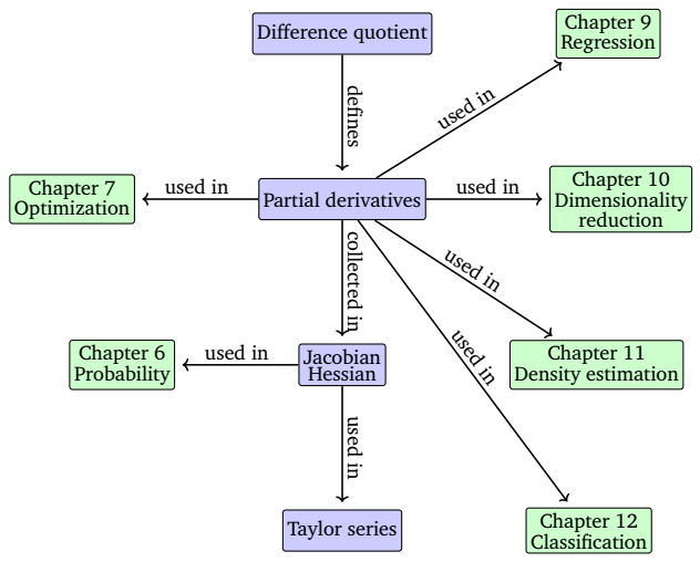
"Mathematics for Machine Learning" fig. 5.2 "mind map".
This says
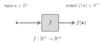
The domain contains allowed inputs
the codomain specifies the output space
the image contains outputs actually attained
$$ f(\mathbb{R}^n) =\{f(\mathbf{x}):\mathbf{x}\in\mathbb{R}^n\} \subseteq\mathbb{R}^m. $$What is it doing?
What are domain, codomain, and image?
Examples:
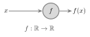
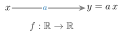
Diagram notation used from here on:
A vector argument is a compact notation for describing a multi-variable function.
\begin{align} f:\mathbb R^n &\rightarrow \mathbb R \notag \end{align}$$f(\mathbf x) = f_1(x_1,x_2,...,x_n)$$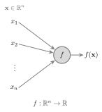
What is $n$ and $\mathbf x$?
What is $\mathbf x$?
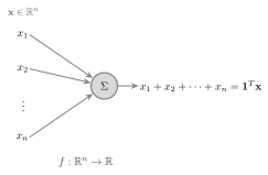
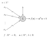
Think of $\mathbf x$ as the variable and $\mathbf a$ as a vector of fixed parameters
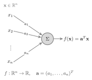
Suppose both $\mathbf x$ and $\mathbf a$ were treated as inputs, what is the domain and codomain of $f(\mathbf x, \mathbf a)$ : $?? \rightarrow ??$
any linear function $\mathbb R^n \rightarrow \mathbb R$ can be described as an inner product
Exercise: prove by using linearity assumption to expand $f(x_1 \mathbf e_1+..+x_n \mathbf e_n)$.
A linear function with an offset
$x$ is a scalar but $f(x)$ is a vector \begin{align} f:\mathbb R &\rightarrow \mathbb R^m \notag \end{align}
$$ f(x) = \begin{pmatrix} f_1(x) \\ f_2(x) \\ \vdots \\ f_m(x) \end{pmatrix} $$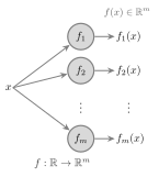
Why can we break up a vector function into scalar functions like this? It didn't work in the other direction (scalar function of vector argument).
Can't separate inputs $$f(\mathbf x) = f(x_1,x_2) = z \ne \text{some combination of } f_1(x_1) \text{ and } f_2(x_2)$$
Can separate outputs $$f(x) = \mathbf z = \begin{pmatrix} z_1 \ z_2
$$
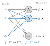
Again note we split up the output into component functions
Vector notation collects multiple scalar inputs or outputs: $$ \mathbf{x}= \begin{pmatrix}x_1\\ \vdots\\ x_n\end{pmatrix}, \qquad f(\mathbf{x})= \begin{pmatrix} f_1(x_1,\ldots,x_n)\\ \vdots\\ f_m(x_1,\ldots,x_n) \end{pmatrix}. $$
| ....................Function type............................................ | .....................Mapping........................... | ....................Example....................... |
|---|---|---|
| Univariate, scalar-valued | $\mathbb{R}\to\mathbb{R}$ | $f(x)=x^2$ |
| Multivariate, scalar-valued | $\mathbb{R}^n\to\mathbb{R}$ | $f(\mathbf{x})=\mathbf{a}^T\mathbf{x}$ |
| Univariate, vector-valued | $\mathbb{R}\to\mathbb{R}^m$ | $f(t)=(\cos t,\sin t)^T$ |
| Multivariate, vector-valued | $\mathbb{R}^n\to\mathbb{R}^m$ | $f(\mathbf{x})=A\mathbf{x}$, $A\in\mathbb{R}^{m\times n}$ |
Here $n$ counts input variables and $m$ counts output variables.
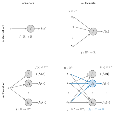
The arrow describes a whole vector, and the box $f$ stands for all $m$ component functions $f_1,\dots,f_m$.
Deep neural networks are often drawn as chains of such boxes.
The most common vector calculus case in optimization, maximize or minimize the objective:
$$ y = f(\mathbf x) = f(x_1,x_2,...,x_n) $$Examples: a metric, regression prediction, or classification, of the collective measurement parameters in $\mathbf x$.
This will be the most common situation in machine learning.
For a multi variable function $f:\mathbb R^n \rightarrow \mathbb R$, i.e. $f(x) = f(x_1,x_2,...,x_n)$,
The $n$ partial derivatives of $f$ are defined as
\begin{align} \dfrac{\partial f}{\partial x_1} &\equiv \lim_{h \rightarrow 0} \dfrac{f(x_1+h,x_2,...,x_n) - f(x_1,x_2,...,x_n)}{h} \notag \\ \vdots \notag \\ \dfrac{\partial f}{\partial x_n} &\equiv \lim_{h \rightarrow 0} \dfrac{f(x_1,x_2,...,x_n+h) - f(x_1,x_2,...,x_n)}{h} \notag \end{align}For scalar function $f(\mathbf x) = f(x_1,x_2,...,x_n)$, the gradient is the vector
$$ \nabla f(x_1,x_2,...,x_n) = \begin{pmatrix} \frac{\partial f}{\partial x_1} \\ \frac{\partial f}{\partial x_2} \\ \vdots \\ \frac{\partial f}{\partial x_n} \end{pmatrix} $$This gives the local slope for each dimension.
Example: if $f(x,y)$ describes the height of the ground. $\nabla f = \left[ \frac{\partial f}{\partial x}, \frac{\partial f}{\partial y}\right]^T$ gives the slope of the ground at every point.
What is the gradient of a function of one variable?
Compute the gradient of $f(x,y)=x^2y + y + 2$ with respect to $x$ and $y$ at the point $(3,4)$
Solve analytically
$$\dfrac{\partial f}{\partial x} = 2xy \;\;\;\;\;\; \dfrac{\partial f}{\partial y} = x^2 + 1$$Example: Compute the gradient of $f(x_1,x_2) = x_1^2 x_2 + x_1 x_2^3$.
Implement solution manually. Requires working out analytically by hand or symbolicly, then implementing the formula.
def f(x,y):
    return x*x*y + y + 2

def df(x,y):
    return 2*x*y, x*x + 1

df(3, 4)
(24, 10)
Solve with PyTorch
Make $x$ and $y$ tensors that track gradients, evaluate $f$, and call backward(). Autograd fills in $\partial f/\partial x$ and $\partial f/\partial y$ at the point where $f$ was evaluated.
x = torch.tensor(3.0, requires_grad=True)
y = torch.tensor(4.0, requires_grad=True)

f(x, y).backward()
df_pytorch = (x.grad, y.grad)
print(df_pytorch)
(tensor(24.), tensor(10.))
Alternatively, torch.autograd.grad(output, inputs) returns the gradients directly, one per input, instead of storing them in .grad. The inputs must have requires_grad=True, and output must be a scalar.
df_pytorch = torch.autograd.grad(f(x, y), [x, y])   # same x, y as above
print(df_pytorch)
(tensor(24.), tensor(10.))
Finite-differences
def fd_derivative_x(f, x, y, eps=0.000001):
    df_x = (f(x + eps,y ) - f(x - eps,y))/(2 * eps)  # partial wrt x
    df_y = (f(x, y + eps) - f(x, y - eps))/(2 * eps) # partial wrt y
    return df_x, df_y

fd_derivative_x(f, 3, 4)
(24.00000000335467, 9.99999999606871)
Note need another finite-difference computation for every variable, so $2n$ total. If $f(\mathbf x)$ slow to compute, this is much slower that manually implemented gradient function $g(\mathbf x) = \nabla f(\mathbf x)$ which is computed 1 time.
The rate of change of a function in any arbitrary direction vector $\mathbf{v}$ (where $\mathbf{v}$ is a unit vector). A scalar:
$$D_{\mathbf{v}} f = \nabla f \cdot \mathbf{v} = |\nabla f| \mathbf u \cdot \mathbf v$$In 2D case, gives slope of surface in direction $\mathbf v$
For what direction $\mathbf v$ is the directional derivative maximized? minimized?
Notation: $\nabla f$ and $\nabla_{\mathbf x} f(\mathbf x)$ are the same column vector; the subscript only names the variable. The directional derivative is written $D_{\mathbf v} f$.
Direct generalization of derivative to higher dimensions.
\begin{align} \frac{d f(\mathbf x )}{d \mathbf x} = \left( \frac{\partial f}{\partial x_1}, \frac{\partial f}{\partial x_2}, ..., \frac{\partial f}{\partial x_n} \right) = \nabla^T_{\mathbf x} f \notag \end{align}Called total derivative because it is taken with respect to all variables (as opposed to partial derivative).
A.k.a, just "derivative", also denoted as $D f(\mathbf x)$ or $d f(\mathbf x)$, and in some texts (M4ML) $\nabla f(\mathbf x)$; here $\nabla f$ always means the column
Convention in this lecture: the gradient $\nabla_{\mathbf x} f$ is a column, the same shape as $\mathbf x$ (like PyTorch's .grad). The derivative $\dfrac{df}{d\mathbf x} = \nabla_{\mathbf x} f^T$ is a row, like a row of the Jacobian.
Texts differ (M4ML uses $\nabla$ for the row). Always keep in mind whether $f$ and $x$ are vectors or scalars (or matrices).
A square matrix containing all second-order partial derivatives of a scalar-valued function. It describes the local curvature of the function's landscape:
$$ H_{ij} = \frac{\partial^2 f}{\partial x_i \partial x_j} $$Example: $f(x,y)=x^2y + y + 2$
$$ \dfrac{\partial^2 f}{\partial x \partial x} = \dfrac{\partial (2xy)}{\partial x} = 2y $$$$ \dfrac{\partial^2 f}{\partial x \partial y} = \dfrac{\partial (2xy)}{\partial y} = 2x $$$$ \dfrac{\partial^2 f}{\partial y \partial x} = \dfrac{\partial (x^2 + 1)}{\partial x} = 2x $$$$ \dfrac{\partial^2 f}{\partial y \partial y} = \dfrac{\partial (x^2 + 1)}{\partial y} = 0 $$Manual Implementation
A single matrix-valued function computation
def d2f(x, y):
    return [2*y, 2*x], [2*x, 0]

d2f(3, 4)
([8, 6], [6, 0])
from torch.autograd.functional import jacobian, hessian

x = torch.tensor(3.0, requires_grad=True)
y = torch.tensor(4.0, requires_grad=True)

def f_vec(v):
    x, y = v
    return x*x*y + y + 2

v0 = torch.tensor([3.0, 4.0])
print('gradient:', jacobian(f_vec, v0))   # Jacobian = total deriv in scalar case
print('Hessian:\n', hessian(f_vec, v0))
gradient: tensor([24., 10.])
Hessian:
 tensor([[8., 6.],
        [6., 0.]])
Differentiate a derivative again in pytorch by keeping its graph
create_graph=True makes the result of torch.autograd.grad differentiable.
x = torch.tensor(5.0, requires_grad=True)
y = x * x

dy_dx, = torch.autograd.grad(y, x, create_graph=True)  # dy/dx = 2x, kept differentiable
d2y_dx2, = torch.autograd.grad(dy_dx, x)               # d2y/dx2 = 2

print(dy_dx, d2y_dx2)
tensor(10., grad_fn=<AddBackward0>) tensor(2.)
For a scalar-valued function of a vector $\mathbf{x}$ evaluated near a point $\mathbf{a}$, the second-order Taylor expansion is $$ f(\mathbf{x}) \approx f(\mathbf{a}) + \nabla f(\mathbf{a})^T (\mathbf{x}-\mathbf{a}) + \frac{1}{2} (\mathbf{x}-\mathbf{a})^T \mathbf{H} (\mathbf{x}-\mathbf{a}) $$ Again the linear approximation is the most commonly used.
Optimization using local linear approximation. Went from too-trivial-to-cover in optimization classes, to the current state-of-the-art due to massive data sizes and parallel computing (scalability)
To minimize an objective $L:\mathbb R^n\rightarrow\mathbb R$, use the linear Taylor approximation at the current point $\mathbf x^{(k)}$,
$$ L(\mathbf x) \approx L(\mathbf x^{(k)}) + \nabla_{\mathbf x}L(\mathbf x^{(k)})^T(\mathbf x-\mathbf x^{(k)}) $$The gradient $\nabla_{\mathbf x}L$ is a vector in the same space as $\mathbf x$. It points in the direction of fastest increase. So step the opposite direction:
$$ \mathbf x^{(k+1)} = \mathbf x^{(k)} - \eta\,\nabla_{\mathbf x}L(\mathbf x^{(k)}), \; \eta>0 $$By the approximation, a small step reduces $L$ by about $\eta\,\|\nabla_{\mathbf x}L\|^2$. At a minimum $\mathbf x^\ast$ the gradient is $\mathbf 0$.
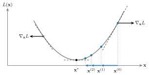
What do we use for the step size $\eta$?
Using the second-order Taylor expansion at $\mathbf x^{(k)}$, with gradient $\nabla_{\mathbf x}L$ and Hessian $\mathbf H$ both evaluated at $\mathbf x^{(k)}$:
$$ L(\mathbf x) \approx L(\mathbf x^{(k)}) + \nabla_{\mathbf x}L^T(\mathbf x-\mathbf x^{(k)}) + \frac{1}{2}(\mathbf x-\mathbf x^{(k)})^T\mathbf H(\mathbf x-\mathbf x^{(k)}) $$Find the minimum of this quadratic approximation by computing its gradient using matrix calculus to get:
$$ \nabla_{\mathbf x}L + \mathbf H(\mathbf x-\mathbf x^{(k)}) $$set this equal to $\mathbf 0$ to get
$$ \mathbf x^{(k+1)} = \mathbf x^{(k)} - \mathbf H^{-1}\nabla_{\mathbf x}L(\mathbf x^{(k)}) $$There is no step size to choose. Each step solves an $n\times n$ linear system, which can get very expensive (if not impossible) for large $n$, but it can take far fewer steps than gradient descent.
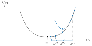
Using partial derivatives with respect to all inputs gives the gradient - the slope of the function over all dimensions,
Using second detivatives, including pairwise combinations between dimensions, gives the curvature of the function, with respect to all dimensions.
These arise in a local Taylor series approximation to the function.
We make use of the local Taylor series in iterative methods for optimization of a scalar objective function.
$f:\mathbb R \rightarrow \mathbb R^m $
$$ \mathbf y(t) = \begin{pmatrix} f_1(t) \\ f_2(t) \\ \vdots \\ f_m(t) \end{pmatrix} $$Examples: a position or velocity vector that changes over time.
back to fundamentals...
$$ f(t) = \begin{pmatrix} f_1(t) \\ f_2(t) \\ \vdots \\ f_n(t) \end{pmatrix} $$\begin{align} \dfrac{d f}{d t} \equiv \lim_{h \rightarrow 0} \dfrac{f(t+h) - f(t)}{h} = ? \end{align}Can view as broadcasting the derivative to all elements: $$ \frac{d}{dt}f(t) = \begin{pmatrix} \frac{d}{dt} f_1(t) \\ \frac{d}{dt} f_2(t) \\ \vdots \\ \frac{d}{dt} f_m(t) \end{pmatrix} $$
Example: $f(t)$ describes position over time in space, while $f'(t)$ describe velocity vector over time.
But note the gradient is also defined as a vector in the prior case with a scalar function of vector argument. Hence we define the total derivative as a row instead. Then we can easily handle the combined case...
What is $\dfrac{df}{dx}$?
As with vector-valued function of scalar argument, we take the derivative of each component function, now in terms of the vector argument $\mathbf x$ instead of $t$.
\begin{align} \frac{d f(\mathbf x )}{d \mathbf x} = \begin{pmatrix}\nabla^T_{\mathbf x} f_1\\ \nabla^T_{\mathbf x} f_2\\ \vdots \\ \nabla^T_{\mathbf x} f_m\end{pmatrix} = \begin{pmatrix} \frac{\partial f_1}{\partial x_1} & \frac{\partial f_1}{\partial x_2} & ... & \frac{\partial f_1}{\partial x_n} \\ \frac{\partial f_2}{\partial x_1} & \frac{\partial f_2}{\partial x_2} & ... & \frac{\partial f_2}{\partial x_n} \\ \vdots & \vdots & & \vdots \\ \frac{\partial f_m}{\partial x_1} & \frac{\partial f_m}{\partial x_2} & ... & \frac{\partial f_m}{\partial x_n} \end{pmatrix} = \mathbf J \notag \end{align}Example: vector fields in physics (gravity, electric field), regression model which predicts a location.
$x\in\mathbb{R}^n$, $y\in\mathbb{R}^m$
| ....Output....... | ..........Input..... | ..........Derivative... | ..................................Example............................. |
|---|---|---|---|
| Scalar | Scalar | $\dfrac{df}{dx}$ | $f(x)=x^2 \implies 2x$ |
| Scalar | Vector | $\dfrac{df}{d\mathbf x}=\nabla^T f$ | $f(\mathbf x)=x_1^2 + x_2^2 \implies \begin{pmatrix}2x_1,& 2x_2\end{pmatrix}$ |
| Vector | Scalar | $\dfrac{dy}{dt}$ | $\mathbf y(t)=\begin{pmatrix}t^2\\3t-t^3\end{pmatrix} \implies \begin{pmatrix}2t\\3-3t^2\end{pmatrix}$ |
| Vector | Vector | $J_{ij}=\frac{\partial y_i}{\partial x_j}$ | $\mathbf y=\begin{pmatrix}x_1^2\\x_1x_2\end{pmatrix} \implies \begin{pmatrix}2x_1 & 0\\ x_2 & x_1\end{pmatrix}$ |
Note the gradient is a column vector, while the derivative of a scalar-valued function with respect to a vector is a row vector ($\nabla_x f^T$).
Basically, the dimensionality of $f$ in rows and the dimensionality of $x$ in columns
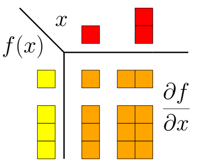
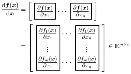
$\mathbf J = \dfrac{df(\mathbf x)}{d\mathbf x}$: the derivative of a vector function, with row $i$ equal to $\nabla^T f_i$.
What is $\dfrac{df(x)}{dx}$?
Matrix-vector product where $A$ is $m \times n$
$$ \frac{d}{d \mathbf x} (\mathbf A \mathbf x) = ? $$For a vector valued function $\mathbf y(\mathbf x)$ with elements $y_i(\mathbf x)$, where $\mathbf x$ has elements $x_j$, the Jacobian is a matrix with $J_{ij} = \dfrac{\partial y_i}{\partial x_j}$.
Plan A: We could build it one row at a time with torch.autograd.grad(y[i], x)
Plan B: use torch.autograd.functional.jacobian, which does this for us.
Exercise: Compute the gradient of $\mathbf A \mathbf x$ for a small system with pytorch.
Affine function of inputs. Also called a Dense layer and fully-connected layer.
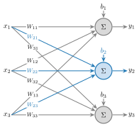
Describe this as a function $f(\mathbf x)$. What is the output vector $\mathbf y$ as a function of $\mathbf x$? What is the Jacobian of $f$?
Suppose you made a linear neural network with the above layer. How would you train it (i.e., chooose $W_{ij}$ and $b_i$)?
import torch

A = torch.tensor([[1., 2., 3.],
                  [4., 5., 6.]])

x = torch.tensor([1., 0., -1.])

# nn.Linear(in, out) computes y = x@A^T + b = (A@x + b).T

layer = torch.nn.Linear(3, 2, bias=False) # weight has shape (out, in) = A's shape
with torch.no_grad():
    layer.weight.copy_(A)

y = layer(x)

print(y)
print(A @ x)
tensor([-2., -2.], grad_fn=<SqueezeBackward4>)
tensor([-2., -2.])
A scalar activation function which is applied elementwise
\begin{align} \boldsymbol{\sigma}(\mathbf x) = \begin{pmatrix}\sigma(x_1)\\ \sigma(x_2)\\ \vdots \\ \sigma(x_n)\end{pmatrix} \end{align}Ex: Assume $\sigma(x)$ is a basic ReLU()
What is the output $\sigma(\mathbf x)$ and its Jacobian for x=[1, -2, 5]
Multiclass classifiers turn a vector of scores $\mathbf z\in\mathbb R^K$ into probabilities
$$p_i = \operatorname{softmax}(\mathbf z)_i = \frac{e^{z_i}}{\sum_{k=1}^K e^{z_k}}$$Unlike an elementwise activation, every output depends on every input, so the Jacobian is not diagonal:
$$\frac{\partial p_i}{\partial z_j} = p_i(\delta_{ij} - p_j) \quad\Rightarrow\quad \mathbf J = \operatorname{diag}(\mathbf p) - \mathbf p\mathbf p^T$$Exercise: derive this with the quotient rule, for the cases $i=j$ and $i\ne j$.
from torch.autograd.functional import jacobian

z = torch.tensor([1.0, 2.0, 0.5])
p = torch.softmax(z, dim=0)

J_autograd = jacobian(lambda z: torch.softmax(z, dim=0), z)
print(J_autograd)


J_formula = torch.diag(p) - torch.outer(p, p)
print('\n',J_formula)
tensor([[ 0.1778, -0.1453, -0.0324],
        [-0.1453,  0.2335, -0.0881],
        [-0.0324, -0.0881,  0.1206]])

 tensor([[ 0.1778, -0.1453, -0.0324],
        [-0.1453,  0.2335, -0.0881],
        [-0.0324, -0.0881,  0.1206]])
A 10-layer network (i.e. pretty small one) will implement a function:
$$f_{9}\Big(f_{8}\big(f_{7}(...f_1(f_0(x)))\big)\Big)$$We use automated applications of the chain rule to optimize these. We can compute its derivative from the derivatives (Jacobians) of each function individually.
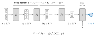
Scalar rules can be extended if careful. Must maintain order now that we are dealing with vectors, matrix multiplication is not commutative in general.
Product rule $\dfrac{d}{dx}\big(f(x)g(x)\big) = \dfrac{df}{dx}\,g(x)+f(x)\,\dfrac{dg}{dx}$
Sum rule $\dfrac{d}{dx}\big(f(x)+g(x)\big) = \dfrac{df}{dx}+\dfrac{dg}{dx}$
Chain rule $\dfrac{d}{dx}\, g\big(f(x)\big) = \dfrac{dg}{df}\,\dfrac{df}{dx}$
When the derivatives are vectors or matrices, the product is a matrix product, taken in the order of the composition. In gradient (column) form the chain rule reads in reverse, as in transposing a product $\nabla_x\, g\big(f(x)\big) = \big(\frac{df}{dx}\big)^T\nabla_f\, g$.
Chain rule for $f(x(t))$, where $x \in \mathbb R^2$ and $t \in \mathbb R$
$f(x(t)) = f(x_1(t),x_2(t))$
Key question, what kind of function is "$x(t)$" here, $\mathbb R^? \rightarrow \mathbb R^?$
Answer: a vector function with a scalar argument. $$x(t) = \begin{pmatrix} x_1(t) \\ x_2(t) \\ \end{pmatrix} $$
Therefore, for first term in $\dfrac{df}{dx}\,\dfrac{dx}{dt}$,
$$\dfrac{df}{dx} =?$$For second term in $\dfrac{df}{dx}\,\dfrac{dx}{dt}$, we have
$$\dfrac{dx}{dt}=?$$Finally, what is the net result $\dfrac{df}{dx}\,\dfrac{dx}{dt}$?
Compute derivative of $f$ wrt $t$ at the point $t = 0$
Consider $f(x(s))$, where $x(s) = \begin{pmatrix} x_1(s) \\ x_2(s) \\ \end{pmatrix} $, and $s = \begin{pmatrix} s_1 \\ s_2 \\ \end{pmatrix}$
$\dfrac{df}{ds} = \dfrac{df}{dx}\,\dfrac{dx}{ds} =?$
Easy part: $\dfrac{df}{dx} = ?$
($f$ is a scalar function)
$\dfrac{df}{ds} = \dfrac{df}{dx}\,\dfrac{dx}{ds} =?$
Hard part: $\dfrac{dx}{ds}=?$
(Both $x$ and $s$ are 2D vectors).
Two linear layers in sequence, with no activation in between ($\mathbf W_1$ is $h\times n$, $\mathbf W_2$ is $m\times h$): $$ \mathbf z = \mathbf W_1\mathbf x + \mathbf b_1, \qquad \mathbf y = \mathbf W_2\mathbf z + \mathbf b_2 $$
Chain rule: the Jacobian of the composition is the product of the Jacobians, in composition order, $$ \frac{d\mathbf y}{d\mathbf x} = \frac{d\mathbf y}{d\mathbf z}\,\frac{d\mathbf z}{d\mathbf x} = \mathbf W_2\,\mathbf W_1 $$ Note sizes work out $(m\times h)(h\times n) = m\times n$
Substituting $\mathbf z$ into $\mathbf y$
$$ \mathbf y = (\mathbf W_2\mathbf W_1)\,\mathbf x + (\mathbf W_2\mathbf b_1 + \mathbf b_2) = \mathbf W'\mathbf x + \mathbf b' $$There is no functional benefit from a deep network of purely linear layers.
from torch.autograd.functional import jacobian

torch.manual_seed(0)
layer1 = torch.nn.Linear(3, 4)
layer2 = torch.nn.Linear(4, 2)

def f(x):
    y = layer2(layer1(x))  # y = W2 (W1 x + b1) + b2
    return y

x = torch.randn(3)
J = jacobian(f, x)
print(J, '\n\n', layer2.weight @ layer1.weight)
tensor([[-0.1577, -0.1227, -0.0054],
        [-0.1189, -0.1485, -0.0592]])

 tensor([[-0.1577, -0.1227, -0.0054],
        [-0.1189, -0.1485, -0.0592]], grad_fn=<MmBackward0>)
A linear layer followed by an activation function $\sigma$ applied element-wise to each output: $$ \mathbf z = \mathbf W\mathbf x + \mathbf b, \qquad \mathbf y = \boldsymbol\sigma(\mathbf z) $$
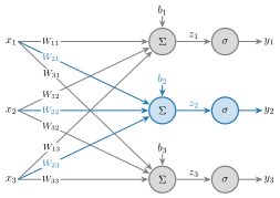
The layer is a composition, so its Jacobian is the product of the two Jacobians we already have, in composition order: $$ \frac{d\mathbf y}{d\mathbf x} = \frac{d\mathbf y}{d\mathbf z}\,\frac{d\mathbf z}{d\mathbf x} = \underbrace{\begin{pmatrix}\sigma'(z_1) & 0 & 0\\ 0 & \sigma'(z_2) & 0\\ 0 & 0 & \sigma'(z_3)\end{pmatrix}}_{\text{activation}}\ \underbrace{\mathbf W}_{\text{linear}}, \qquad \frac{\partial y_i}{\partial x_j} = \sigma'(z_i)\,W_{ij} $$
Later: For a scalar $L$ computed from $\mathbf y$, the gradient is the transpose, so the order reverses: first the activation Jacobian, then the linear one, $$ \nabla_{\mathbf x}L = \Big(\frac{d\mathbf y}{d\mathbf x}\Big)^T\nabla_{\mathbf y}L = \mathbf W^T\,\mathrm{diag}\big(\sigma'(\mathbf z)\big)\,\nabla_{\mathbf y}L $$ Working backward from $L$ one layer at a time like this is backpropagation.
Take the derivative of the least-squares "loss" and set it equal to zero
\begin{align} L(\boldsymbol\beta) &= \Vert\mathbf y - \mathbf X\boldsymbol\beta\Vert_2^2 \notag \\ & = (\mathbf y - \mathbf X\boldsymbol\beta)^T(\mathbf y - \mathbf X\boldsymbol\beta) \notag \\ &= \mathbf y^T \mathbf y + \boldsymbol\beta^T \mathbf X^T \mathbf X \boldsymbol\beta -2 \boldsymbol\beta ^T \mathbf X \mathbf y \notag \\ \end{align}Compute the gradient using matrix calculus
$$\nabla_{\boldsymbol\beta} L = -2\mathbf X^T(\mathbf y - \mathbf X\boldsymbol\beta)$$Setting the gradient to zero gives the normal equations $$ \mathbf X^T\mathbf X\boldsymbol\beta = \mathbf X^T\mathbf y $$
Solving directly gives the pseudoinverse.
from sklearn.datasets import load_diabetes
from sklearn.linear_model import LinearRegression

X, y = load_diabetes(return_X_y=True)
X1 = np.column_stack([np.ones(len(X)), X])     # column of ones for the intercept

beta = np.linalg.solve(X1.T @ X1, X1.T @ y)    # normal equations

lin = LinearRegression().fit(X, y)
print('intercept:', beta[0], lin.intercept_, '  coefficients:', beta[1:], lin.coef_)
intercept: 152.13348416289597 152.13348416289597   coefficients: [ -10.0098663  -239.81564367  519.84592005  324.3846455  -792.17563855
  476.73902101  101.04326794  177.06323767  751.27369956   67.62669218] [ -10.0098663  -239.81564367  519.84592005  324.3846455  -792.17563855
  476.73902101  101.04326794  177.06323767  751.27369956   67.62669218]
Data $\mathbf X$ ($N$ patients $\times$ $D$ features), centered so each column has mean zero. Summarize each patient by one number, a linear score of the features with weights $\mathbf w\in\mathbb R^D$:
$$s_i = \mathbf x_i^T\mathbf w = w_1 x_{i1} + \cdots + w_D x_{iD}, \qquad \mathbf s = \mathbf X\mathbf w$$A score that is nearly the same for every patient tells us nothing; a good one should spread the patients out.
Choose $\mathbf w$ to maximize the variance of the scores.
Because the features are centered, so are the scores
$$ \bar s = \bar{\mathbf x}^T\mathbf w = \mathbf 0^T \mathbf w = 0 $$So the variance is the mean square:
$$\operatorname{Var}(s) = \frac1N\sum_i s_i^2 = \frac1N\,\mathbf s^T\mathbf s = \frac1N(\mathbf X\mathbf w)^T(\mathbf X\mathbf w) = \mathbf w^T\Big(\underbrace{\tfrac1N\mathbf X^T\mathbf X}_{\boldsymbol\Sigma}\Big)\mathbf w$$$\boldsymbol\Sigma$ is the covariance matrix of the features. The variance of the score is a quadratic form in $\mathbf w$
The first principal direction is the unit vector that captures the most variance:
$$\max_{\mathbf w}\; \mathbf w^T\boldsymbol\Sigma\mathbf w \quad\text{subject to}\quad \mathbf w^T\mathbf w = 1$$The scale of $\mathbf w$ is meaningless (the relative contribution of features is what matters), so we chose $\Vert\mathbf w\Vert = 1$
Lagrangian: $$\mathcal L(\mathbf w,\lambda) = \mathbf w^T\boldsymbol\Sigma\mathbf w - \lambda(\mathbf w^T\mathbf w - 1)$$
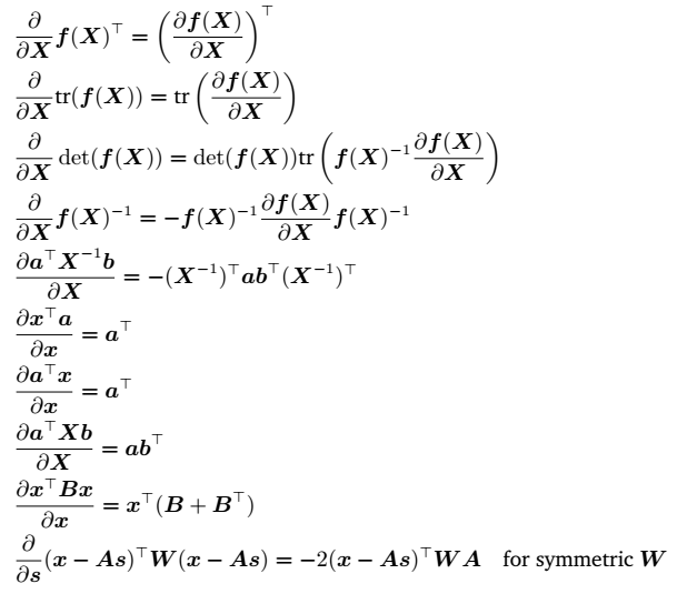
Using $\nabla_{\mathbf w}(\mathbf w^T\mathbf A\mathbf w) = (\mathbf A + \mathbf A^T)\mathbf w$ from matrix calculus, plus the symmetry of $\boldsymbol\Sigma$:
$$\nabla_{\mathbf w}\mathcal L = 2\boldsymbol\Sigma\mathbf w - 2\lambda\mathbf w = 0 \quad\Rightarrow\quad \boldsymbol\Sigma\mathbf w = \lambda\mathbf w$$So $\mathbf w$ is an eigenvector of $\boldsymbol\Sigma$. The variance it captures is $\mathbf w^T\boldsymbol\Sigma\mathbf w = \lambda\,\mathbf w^T\mathbf w = \lambda$, largest for the top eigenvalue. The second principal direction maximizes the same variance among unit vectors orthogonal to the first, and so on down the eigenvalues.
from sklearn.datasets import load_breast_cancer
from sklearn.preprocessing import StandardScaler
from sklearn.decomposition import PCA

X = StandardScaler().fit_transform(load_breast_cancer().data)   # centered (and scaled)
Sigma = X.T @ X / X.shape[0]

evals, evecs = np.linalg.eigh(Sigma)   # eigenvalues in ascending order
w = evecs[:, -1]                       # eigenvector of the largest eigenvalue

pc1 = PCA(n_components=1).fit(X).components_[0]
#print(abs(w @ pc1))
print('variance captured:', w @ Sigma @ w, '  top eigenvalue:', evals[-1])
variance captured: 13.281607682257905 top eigenvalue: 13.281607682257917
Add the penalty $\lambda\Vert\boldsymbol\beta\Vert_2^2$. The gradient gains a $2\lambda\boldsymbol\beta$ term, so
$$(\mathbf X^T\mathbf X + \lambda\mathbf I)\boldsymbol\beta = \mathbf X^T\mathbf y$$scikit-learn does not penalize the intercept, so center $\mathbf X$ and $\mathbf y$ and leave the intercept out of the penalized system.
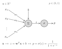
An affine function followed by the sigmoid, $\mathbb R^n\to\mathbb R\to(0,1)$. It is a composition, so the chain rule gives how $p$ changes with $\mathbf w$.
Each patient gets a predicted probability $p_i = \sigma(\mathbf x_i^T\mathbf w)$ of the outcome (here, a malignant tumor), and we observe $y_i\in\{0,1\}$.
A practical requirement, the same observed-versus-expected check used for any clinical risk score: the model should predict as many cases as were observed, in total and weighted by each feature,
$$\mathbf u(\mathbf w) = \mathbf X^T(\mathbf y - \mathbf p) = \mathbf 0$$one equation per column of $\mathbf X$. The column of ones gives $\sum_i y_i = \sum_i p_i$: total observed cases = total expected cases.
$\mathbf u$ is a vector-valued function of $\mathbf w$, and nonlinear because of $\sigma$, so there is no closed form. Linearize with its Jacobian and solve for the step: $\mathbf u(\mathbf w+\boldsymbol\Delta)\approx\mathbf u(\mathbf w)+\mathbf J\boldsymbol\Delta=\mathbf 0$.
By the chain rule, with the diagonal Jacobian of the elementwise sigmoid,
$$\mathbf J = \frac{\partial\mathbf u}{\partial\mathbf w} = -\mathbf X^T\frac{\partial\mathbf p}{\partial\mathbf w} = -\mathbf X^T\mathbf S\mathbf X,\qquad \mathbf S = \operatorname{diag}\big(p_i(1-p_i)\big)$$$$\mathbf w \leftarrow \mathbf w + (\mathbf X^T\mathbf S\mathbf X)^{-1}\mathbf X^T(\mathbf y-\mathbf p)$$Each step is a weighted least-squares solve, so statisticians call this iteratively reweighted least squares (IRLS). The weight $p_i(1-p_i)$ is the variance of patient $i$'s 0/1 outcome: patients whose outcome is least certain ($p_i$ near 0.5) count the most.
from sklearn.datasets import load_breast_cancer
from sklearn.preprocessing import StandardScaler
from sklearn.linear_model import LogisticRegression

Xb, yb = load_breast_cancer(return_X_y=True)
ym = 1 - yb                                      # 1 = malignant (scikit-learn codes benign as 1)
Xb = StandardScaler().fit_transform(Xb)[:, :5]   # 5 features: all 30 nearly separate the classes and the fit diverges
X1 = np.column_stack([np.ones(len(Xb)), Xb])

sigmoid = lambda z: 1 / (1 + np.exp(-z))

w = np.zeros(X1.shape[1])
for it in range(10):                             # Newton's method on u(w) = X^T (y - p) = 0
    p = sigmoid(X1 @ w)
    u = X1.T @ (ym - p)                          # observed minus expected, one entry per column of X
    XtSX = X1.T @ (X1 * (p * (1 - p))[:, None])  # -Jacobian of u, without forming the N x N matrix S
    w = w + np.linalg.solve(XtSX, u)
    print(it, f'observed cases {ym.sum()}, expected {p.sum():.2f}, |u| = {np.linalg.norm(u):.2e}')

logr = LogisticRegression(penalty=None).fit(Xb, ym) # scikit learn version
w, np.r_[logr.intercept_, logr.coef_[0]]
0 observed cases 212, expected 284.50, |u| = 3.85e+02
1 observed cases 212, expected 226.59, |u| = 1.11e+02
2 observed cases 212, expected 215.64, |u| = 4.26e+01
3 observed cases 212, expected 211.94, |u| = 1.62e+01
4 observed cases 212, expected 211.07, |u| = 6.13e+00
5 observed cases 212, expected 211.52, |u| = 2.06e+00
6 observed cases 212, expected 211.94, |u| = 2.87e-01
7 observed cases 212, expected 212.00, |u| = 5.79e-03
8 observed cases 212, expected 212.00, |u| = 2.39e-06
9 observed cases 212, expected 212.00, |u| = 3.90e-13
/opt/venv/lib/python3.12/site-packages/sklearn/linear_model/_logistic.py:1381: FutureWarning: 'penalty' was deprecated in version 1.8 and will be removed in 1.10. To avoid this warning, leave 'penalty' set to its default value and use 'l1_ratio' or 'C' instead. Use l1_ratio=0 instead of penalty='l2', l1_ratio=1 instead of penalty='l1', l1_ratio set to a float between 0 and 1 instead of penalty='elasticnet', and C=np.inf instead of penalty=None.
  warnings.warn(
(array([  0.45924555, -22.09485226,   1.56463237,  14.7403169 ,
         14.68921315,   1.66460148]),
 array([  0.46112047, -22.09209605,   1.56528365,  14.72348074,
         14.70887019,   1.66571615]))
see also