BDS 761: Data Science and Machine Learning I

$\Omega$ = set of all possible outcomes of an experiment
Examples:
By definition (here) different outcomes are mutually exclusive
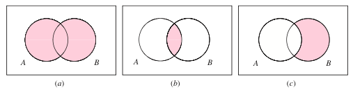
subset of the sample space. That is, any collection of outcomes forms an event.
Example:
Toss a coin twice. Sample space: $\Omega = \{HH, \ HT, \ TH, \ TT\}$
Let event $A$ be the event that there is exactly one head, then $A = \{HT, \ TH \}$
$A$ is a subset of $\Omega$, and we write $A \subset \Omega$
Notation note: $P(A,B) = P(A \text{ AND } B) = P(A \cap B)$
Assuming we define the outcomes of an experiment as distinct events $\Omega = \{x_1, \ x_2, ..., \ x_n\}$
$$P(x_1\cup x_2 \cup \dots \cup x_n) = P(x_1) + P(x_2) + \dots + P(x_n)$$Tukey 1947(?)
Shannon "A mathematical theory of information", 1948.
Computers - count of Binary Digits. 01101011 ~ 8-bit value (byte)
Information Theory - a measure of minimum number of bits needed to represent the information.
Consider 8 random coin flips. Represent result with 8 binary numbers.
But what if the coin is biased? Or we get digits according to some other distribution?
Consider 3-bit number example. The possible values are 000, 001, 010, 011, 100, 101, 110, 111 $\rightarrow$ $2^3 = 8$ possibilities.
Recall the definition of the log: $$ b^y = x \quad \Longleftrightarrow \quad \log_b(x) = y $$
$2^3 = 8 \Rightarrow \log_2(8) = 3.$
$2^8 = 256 \Rightarrow \log_2(256) = 8.$
Other handy facts:
For a discrete random variable $X$ with possible outcomes $\Omega = \{ x_1, x_2, ..., x_n \}$, which have probabilities $p_i$, the information in a measurement which gives outcome $x_i$ is:
$$ I(x_i) = -\log_2 P(X=x_i) $$The units of information are bits.
Also sometimes called self-information to distinguish from general use of term and other quantities such as Fisher Information
Suppose we have one "bit" of data that can be either 0 or 1, i.e. $X \in \{0, 1\}.$
If the bit is perfectly random both outcomes equally likely, so:
$$P(X=0) = P(X=1) = \tfrac{1}{2}.$$$$ \tfrac{1}{2} = 2^{-1} \rightarrow \log_2 \tfrac{1}{2} = -1 \rightarrow I(X) = - \log_2 \tfrac{1}{2} = 1 $$Each outcome gives 1 bit of information when observed:
since $0\le P \le 1$, $I\ge 0$.
High $P$ outcomes: there's small $I$, not big news. It's a fact, often not worth recording because it's almost always true. Don't devote much space to such details.
Low $P$ outcomes: get large $I$, more storage/transmission should be used. Stores only most pertinent outcomes you wouldn't have just guessed.
Ex: record fact that patient is an amputee when true, but not fact that patient is not an amputee otherwise.
suppose $P(X=1) = 0.9, \; P(X=0) = 0.1.$
Then if you observe $X=1$, you learn less because it was already likely. If you observe $X=0$, you learn more because it was surprising.
Choice of base amounts to a scale factor $$ \log_b x=\frac{\log_a x}{\log_a b} \propto \log_a x $$
The log is monotonic $\log(x) > \log(y)$ if and only if $x>y$.
The log is strictly concave $\rightarrow$ $\ln(tx + (1-t)y) \geq t\ln(x) + (1-t)\ln(y)$
Tiny numbers become big negative numbers, reducing underflow in calculations.
The above makes it very handy in optimization and numerical computation to work with log values rather than original parameters, which can be confusing. Hence the value of thinking in terms of information.
Events A and B are independent if and only if: $P(A \cap B) = P(A)P(B)$
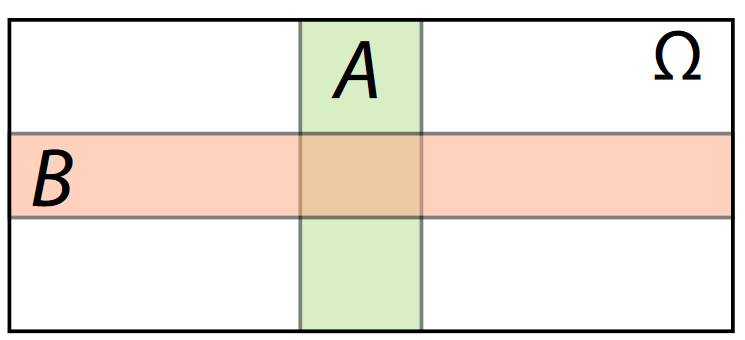
so $I(A \cap B) = -\log(P(A)P(B)) = -\log(P(A)) + -\log(P(B)) = I(A)+I(B)$ -- information adds when independent.
For dependent variables, the information is redundant, maybe we gain little or no new information from more
How surprising is it to get heads (give in units of bits)? $P(H)$
How surprising is the number 0011?
Consider an event which is 4 independent coin flips of a fair coin resulting in 0011.
Compute the information for events with probability 0, 1, 0.5, 0.9, 0.1
Recall that for any positive $x$ and bases $a,b>1$, $$ \log_b x=\frac{\log_a x}{\log_a b}. $$ The change of base is multiplication by a constant: $$ \log_b x = c,\log_a x,\qquad c=\frac{1}{\log_a b}. $$ All log-values in base $a$ are just rescaled to obtain base $b$.
Thus the choice of base can be viewed as a choice of units. For information, the units for base 2 are bits, while units for base $e$ are called nats.
Compute the conversions between bits and nats.
If an event has probability $p = \tfrac{1}{256} = 2^{-8}$, $ I = -\log_2(p) = 8\ \text{bits.} $
This means observing the event resolves one of $2^8 = 256$ equally likely possibilities.
Think of an 8-bit variable $(X_1,X_2, ...,X_8)$ as a sequence of binary decisions:
Is $X_2$ = 0 or 1? -> another bit
...
Is $X_8$ = 0 or 1? -> 8th bit
Each independent bit halves the uncertainty. After 8 such halvings: $$ 1 / 2^8 = 1 / 256. $$ So knowing all 8 resolves all uncertainty among 256 possibilities.
For binary test
$$\text{odds} = \dfrac{P(A)}{1-P(A)} = \dfrac{P(A)}{P(\text{not} A)}$$If $B_1, B_2, \dots, B_k$ form a partition of $\Omega$, then $(A \cap B_1), (A \cap B_2), \dots, (A \cap B_k)$ form a partition of the set or event A.
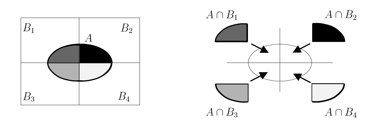
The probability of event A is therefore the sum of its parts:
$$P(A) = P(A \cap B_1) + P(A \cap B_2) + P(A \cap B_3) + P(A \cap B_4)$$But what happens to information in this case?
Joint probability : $P(A \cap B) = P(A|B) \times P(B)$
Interpret in terms of information
If $B_1, \dots, B_k$ partition $S$, then for any event A,
$$ P(A) = \sum_{i = 1}^k P(A \cap B_i) = \sum_{i = 1}^k P(A | B_i) P(B_i) $$We can write any joint probability as incremental product of conditional probabilities,
$ P(A_1 \cap A_2) = P(A_1)P(A_2 | A_1) $
$ P(A_1 \cap A_2 \cap A_3) = P(A_1)P(A_2 | A_1)P(A_3 | A_2 \cap A_1) $
In general, for $n$ events $A_1, A_2, \dots, A_n$, we have
$ P (A_1 \cap A_2 \cap \dots \cap A_n) = P(A_1)P(A_2 | A_1) \dots P(A_n | A_{n-1} \cap \dots \cap A_1) $
.. in terms of information
$$I(A \cap B) = I(A|B) + I(B)$$$$I(A|B) + I(B) = I(B|A) + I(A)$$Probability basic concepts, axioms
Joint probability $P(A \cap B) = P(A|B) \times P(B)$
Bayes Law $ P(A|B) = \frac{P(B|A) \times P(A)}{P(B)}$
Chain Rule for Probability
$ P (A_1 \cap A_2 \cap \dots \cap A_n) = P(A_1)P(A_2 | A_1) \dots P(A_n | A_{n-1} \cap \dots \cap A_1) $
Law of total probability $P(A) = P(A \cap B_1) + P(A \cap B_2) + P(A \cap B_3) + P(A \cap B_4)$ where $B_i$ partition set of all possible outcomes
Notation shorthands $P(A \cap B) = P(A,B) = P(A \text{ AND } B)$
If the outcome is random, we don’t know which event we’ll see; we can only compute the expected information gain: $$ H(X) = \mathbb{E}[I(X)] = -\sum_x P(x) \log_2 P(x). $$
This is the Shannon entropy of the distribution.
For a fair coin: $$ H = -0.5\log_2 0.5 - 0.5\log_2 0.5 = 1 \text{ bit.} $$
For a biased coin $p=0.9$ or $0.1$ $$ H = -0.9\log_2 0.9 - 0.1\log_2 0.1 \approx 0.469 \text{ bits.} $$
The average number of bits needed to represent the outcome is smaller when one value is much more probable
The effective number of outcomes from some average information. E.g. if coin was fair.
$$ \text{Perp}(P) = 2^{H(P)}$$Work backwards using previous entropies.
Number of possible states = $2^8 = 256$ = Distinct configurations of 8 binary variables
Probability of one state = $p = \frac{1}{256} = 2^{-8}$ = Chance of each pattern (if uniform)
Information = $I = -\log_2(2^{-8}) = 8$ = “How many binary questions to identify this state”
Entropy = $H = 8\text{ bits}$ = Average information before observing the value
Perplexity = $\text{Perp}(P) = 2^{H} = 2^8 = 256$
Variable $X=(X_1,\dots,X_8)$ with 8 "bits", meaning variables with possible outcomes $\Omega = \{0,1\}$
$$ X_i\sim \mathrm{Bernoulli}(\theta_i)\;\; \rightarrow \; \Pr(X_i=1)=\theta_i,\ \Pr(X_i=0)=1-\theta_i. $$For a single Bernoulli bit we have entropy
$$ H_b(\theta)=-\theta\log_2\theta-(1-\theta)\log_2(1-\theta)\quad\text{(bits)}. $$And assuming all bits are independent and have the same $\theta_i
$$ H(X)=\sum_{i=1}^8 H_b(\theta_i) = 8 H_b(\theta) $$with $H(X)\in [0,8]$ bits, maximized at $\theta=\tfrac{1}{2}$, the uniform 8-bit case.
Kullback–Leibler (K-L) divergence measures how one probability distribution $Q(x)$ diverges from another $P(x)$ that represents the “true” or reference distribution. For the discrete case:
$$ D_{KL}(P \parallel Q) = \sum_i P(X=x_i) \log \frac{P(X=x_i)}{Q(X=x_i)} $$express this in terms of information
"Cross-Entropy" term: $\;\;\; H(P, Q) = -\mathbb{E}_P[\log Q] = -\sum_i P(X=x_i) \log Q(X=x_i) $
How does the K-L Divergence relate to the information?
We write it simply as $$ D_{KL}(P \parallel Q) = \sum_x P(x) \log \frac{P(x)}{Q(x)} $$
Suppose a biased coin actually has
$$ P(\text{Heads}) = 0.9,\quad P(\text{Tails}) = 0.1 $$but your model is $$ Q(\text{Heads}) = 0.5,\quad Q(\text{Tails}) = 0.5 $$
Compute K-L divergence between distributions $P$ and $Q$.
For a discrete variable $X$, entropy is the expected number of bits needed to describe an outcome:
$$ H(X) = -\sum_x P(x)\log_2 P(x) $$A continuous variable has a probability density $p(x)$ instead of a probability mass. The same formula with an integral defines the differential entropy:
$$ h(X) = -\int p(x)\log p(x)\,dx = \mathbb{E}\left[-\log p(X)\right] $$It is still the expected surprise per observation.
Entropy measures how uncertain a distribution is. Fisher information measures how sharply the distribution changes with a parameter $\theta$. It is written $\mathcal{I}(\theta)$, not to be confused with the information $I(x)$.
For a model $p(x\mid\theta)$, the derivative of the log-likelihood is called the score. The Fisher information is its expected square:
$$ \mathcal{I}(\theta) = \mathbb{E}\left[\left(\frac{\partial}{\partial\theta}\ln p(X\mid\theta)\right)^2\right] = -\mathbb{E}\left[\frac{\partial^2}{\partial\theta^2}\ln p(X\mid\theta)\right] $$The second form (valid given regularity conditions) is the expected curvature of the log-likelihood.
| ......Concept........ | ..............Definition................................ | ............Measures.................... |
|---|---|---|
| Self-information | $I(x) = -\log p(x)$ | Surprise of one outcome |
| Entropy | $H(X) = -\sum_x p(x)\log p(x)$ | Expected surprise, discrete |
| Differential entropy | $h(X) = -\int p(x)\log p(x)\,dx$ | Expected surprise, continuous |
| Fisher information | $\mathcal{I}(\theta) = \mathbb{E}\left[(\partial_\theta \ln p(X\mid\theta))^2\right]$ | Precision about a parameter |
All are in bits except FI which is in inverse parameters units
One of most popular and widely used algorithms in industry.
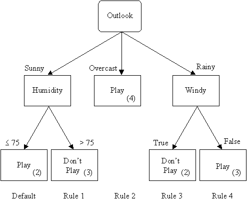
Combines a tree of simple classifiers (the nodes) to make big sophisticated classifier
How to predict with a decision tree it pretty clear: you just answer the questions and follow the path to the appropriate leaf node. But how do we build a decision tree? How do we determine which feature we should split on? This is the crux of the decision tree algorithm.
Focus on algorithms that only use binary decisions ("splits"). Can make any variable binary:
We have a bunch of features somehow, can be anything
Need to convert some of these to binary splits
In order to pick which feature to split on, we need a way of measuring how good the split is. This is what information gain is for.
The entropy of a set is a measure of the amount of disorder. Intuitively, if a set has all the same labels, that'll have low entropy and if it has a mix of labels, that's high entropy. We would like to create splits that minimize the entropy in each size. If our splits do a good job splitting along the boundary between classes, they have more predictive power.
Definition:
$$ H(S) = - \sum_{c_i \in S} P(c_i) \ln(P(c_i)) $$$P(c_i)$ = Probability of class
$P(c_i)$ = Probability of class
Relative Frequency ~ percent of the data that belongs to the class
$$ P(c_i) = \frac{\text{number samples in class i}}{\text{total number of samples in all classes}} $$Prior belief
$$ P(c_i) = \text{fraction of samples we expect to be in class i, based on science etc.} $$Entropy of the set depends on how spread probability is among different classes: $$ H(S) = - \sum_{c_i \in S} P(c_i) \ln(P(c_i)) $$
a dataset of coin-flip outcomes (consider actual data, and theoretically)
the population, separated into classes according to being healthy or having a disease that only afflicts one percent of the population
If you have a collection of datapoints, the entropy will be large when they are evenly distributed across the classes and small when they are mostly the same class.
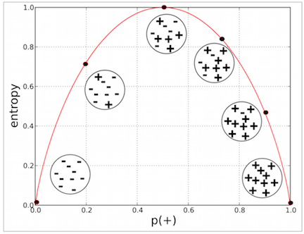
So we would like splits that minimize entropy. Consider why.
We use information gain to determine the best split:
$$ Gain(S,D) = H(S) - \sum_{V \in D} \frac{|V|}{|S|}H(V) $$$S$ is the original set and $D$ is the splitting of the set (a partition).
Each $V$ is a subset of $S$. All of the $V$'s are disjoint and make up $S$.
Given the population, separated into classes according to being healthy or having a disease that only afflicts one percent of the population
Split out a subset with a positive test outcome, for test that has a 50 percent false positive rate
Alternative way of measuring which split is the best. It's a measure of this probability:
To build our tree, we use a brute force method. We try every possibility for splitting at each node and choose the one with the best information gain. Here's the pseudocode for building a Decision Tree:
# def BuildTree:
#    If every item in the dataset is in the same class or there is no feature left to split the data:
#        return a leaf node with the class label
#    Else:
#        1. find the best feature and value to split the data
#        2. split the dataset
#        3. create a node:
#        4. for each split:
#                 call BuildTree and add the result as a child of the node
#        5. return node
from sklearn import tree
X = [[0, 0], [1, 1]]
Y = [0, 1]
clf = tree.DecisionTreeClassifier()
clf = clf.fit(X, Y) # TRAINING
After being fitted, the model can then be used to predict the class of samples:
clf.predict([[2., 2.]])
array([1])
Alternatively, the probability of each class can be predicted, which is the fraction of training samples of the same class in a leaf
clf.predict_proba([[2., 2.]])
array([[0., 1.]])
XGBoost, LightGBM and scikit-learn's HistGradientBoosting* are the leading models in kaggle competitions with tabular data
The model is a sum of small regression trees, each one correcting the errors left by the ones before it:
$$F_M(\mathbf x) = F_0 + \eta\,h_1(\mathbf x) + \eta\,h_2(\mathbf x) + \cdots + \eta\,h_M(\mathbf x)$$Where the corrections come from is a gradient with respect to a vector.
A regression tree predicts a number by asking a short sequence of yes/no questions about the features:
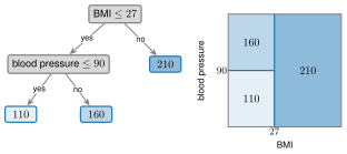
The result is a step function of $\mathbf x$ (right): one constant on each rectangle of the feature space. In boosting the tree is fitted to the residuals $r_i$, so each leaf predicts a mean residual.
A regression tree is a step function: one constant per leaf, chosen by the sequence of splits. For the tree above, with $\mathbf x = (\text{BMI}, \text{BP})$,
$$ F(\mathbf x) = \begin{cases} 110 & \text{if } \text{BMI} \le 27 \text{ and } \text{BP} \le 90 \\ 160 & \text{if } \text{BMI} \le 27 \text{ and } \text{BP} > 90 \\ 210 & \text{if } \text{BMI} > 27 \end{cases} $$Collect the predictions for the $N$ training patients in a vector and measure the fit by the squared error:
$$\mathbf F = \big(F(\mathbf x_1),\dots,F(\mathbf x_N)\big)^T\in\mathbb R^N, \qquad E(\mathbf F) = \tfrac12\Vert\mathbf y-\mathbf F\Vert^2 = \tfrac12\sum_i (y_i-F_i)^2$$$E:\mathbb R^N\to\mathbb R$ is a scalar function of a vector, with gradient
$$\nabla_{\mathbf F}E = -(\mathbf y-\mathbf F) = -\mathbf r$$The negative gradient is the vector of residuals $\mathbf r$: the fastest way to reduce the squared error is to move each prediction toward its target.
A plain gradient step $\mathbf F\leftarrow\mathbf F+\eta\,\mathbf r$ only changes the predictions at the training points (and with $\eta=1$ it simply copies $\mathbf y$). Boosting instead fits a small tree $h$ to $\mathbf r$, so the step also applies to new patients.
The same loop on scikit-learn's diabetes data (10 baseline measurements, disease progression after one year), with depth-3 trees, checked against GradientBoostingRegressor and compared with linear regression on held-out patients.
from sklearn.datasets import load_diabetes
from sklearn.ensemble import GradientBoostingRegressor
from sklearn.linear_model import LinearRegression
from sklearn.model_selection import train_test_split
from sklearn.tree import DecisionTreeRegressor
import numpy as np

X, y = load_diabetes(return_X_y=True)
Xtr, Xte, ytr, yte = train_test_split(X, y, random_state=0)

eta = 0.1
n_trees = 100
F_tr, F_te = np.full(len(ytr), ytr.mean()), np.full(len(yte), ytr.mean())
mse_tr, mse_te = [], []
for m in range(n_trees):
    r = ytr - F_tr   # residuals = negative gradient of the squared error
    h = DecisionTreeRegressor(max_depth=3, random_state=0).fit(Xtr, r)
    F_tr += eta * h.predict(Xtr)
    F_te += eta * h.predict(Xte)
    mse_tr.append(np.mean((ytr - F_tr) ** 2))
    mse_te.append(np.mean((yte - F_te) ** 2))

gbr = GradientBoostingRegressor(n_estimators=n_trees, learning_rate=eta, max_depth=3, random_state=0).fit(Xtr, ytr)

print(' MSE: boosting from scratch:             %.1f' % mse_te[-1])
print(' MSE: sklearn GradientBoostingRegressor: %.1f' % np.mean((yte - gbr.predict(Xte)) ** 2))
 MSE: boosting from scratch:             3879.3
 MSE: sklearn GradientBoostingRegressor: 3898.2
# more trees always lower the training error; the test error tells us when to stop

figure(figsize=(5, 3))
plot(mse_tr, label='boosting, train'); plot(mse_te, label='boosting, test')
axhline(lin_mse, color='gray', ls='--', label='linear regression, test')
xlabel('number of trees'); ylabel('MSE'); legend();

# step size: smaller steps need more trees but usually reach a lower test error

figure(figsize=(5, 3))
for eta_k in [1.0, 0.3, 0.1]:
    F_tr, F_te, curve = np.full(len(ytr), ytr.mean()), np.full(len(yte), ytr.mean()), []
    for m in range(200):
        h = DecisionTreeRegressor(max_depth=3, random_state=0).fit(Xtr, ytr - F_tr)
        F_tr += eta_k * h.predict(Xtr)
        F_te += eta_k * h.predict(Xte)
        curve.append(np.mean((yte - F_te) ** 2))
    plot(curve, label=f'eta = {eta_k}')
axhline(lin_mse, color='gray', ls='--', label='linear regression')
xlabel('number of trees'); ylabel('test MSE'); legend();

"(Student-) t-distributed Stochastic Neighbor Embedding"
Targets 2D or 3D embeddings for visualization
Balances local and global structure by minimizing K-L Divergence between distribution for each.
https://scikit-learn.org/stable/modules/generated/sklearn.manifold.TSNE.html
"Visualizing High-Dimensional Data Using t-SNE", van der Maaten and Hinton, JMLR 2008.
For points $x_i\in\mathbb{R}^D$:
Model high-dimensional similarities with Gaussian kernels $$ p_{j|i}=\frac{\exp(-|x_i-x_j|^2/2\sigma_i^2)}{\sum_{k\neq i}\exp(-|x_i-x_k|^2/2\sigma_i^2)} $$
Choose desired Perp of $p_{j|i}$ as input parameter, and $\sigma_i^2$ is chosen to achieve this. Then for symmetrized distribution:
$$ p_{ij}=\frac{p_{i|j}+p_{j|i}}{2N}. $$
Model low-dimensional similarities for embedded points $y_i\in\mathbb{R}^2$ using Student-t kernels $$ q_{ij}=\frac{(1+|y_i-y_j|^2)^{-1}}{\sum_{k\neq l}(1+|y_k-y_l|^2)^{-1}}. $$
Student-t distribution has heavy tails to avoid overly-clustering data. Also convenient choice for optimization complexity.
Optimize over embedded points by minimizing KL divergence between these distributions. $$ \mathrm{KL}(P|Q)=\sum_{i\neq j} p_{ij}\log\frac{p_{ij}}{q_{ij}}. $$
from sklearn.manifold import TSNE
#help(TSNE)
import numpy as np
from sklearn.manifold import TSNE
import matplotlib.pyplot as plt

# toy dataset: three tight clusters in 2D, then embedded to 10D
rng = np.random.default_rng(0)
A = rng.normal([0,0], 0.1, (50,2))
B = rng.normal([3,0], 0.1, (50,2))
C = rng.normal([0,3], 0.1, (50,2))
X2 = np.vstack([A,B,C])

# map to 10D with a random linear transform
W = rng.normal(size=(2,10))
X10 = X2 @ W

# t-SNE back to 2D
Y = TSNE(n_components=2, perplexity=20, learning_rate=200,
         init="random", random_state=0).fit_transform(X10)

plt.scatter(Y[:,0], Y[:,1], c=np.repeat([0,1,2], 50), s=20)
plt.title("Toy t-SNE example")
plt.show()