BDS 761: Data Science and Machine Learning I

References
the task of assigning a label or category to an entire text or document
Feature Representation of input ~ $\mathbf x$ vector, $x_i = $ feature $i$
Classification function that computes $P(y|\mathbf x)$
Loss function (a.k.a, Cost) for learning, i.e. optimization objective such as squared error
Training algorithm for optimizing objective. E.g., Stochastic Gradient Descent.
Training - run training algorithm to optimize model
Test - compare model performance to true labels on held-out set
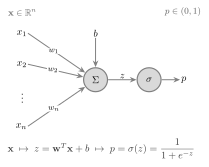
(a neural network can be viewed as a series of logistic regression classifiers stacked on top of each other.)
NFL Example
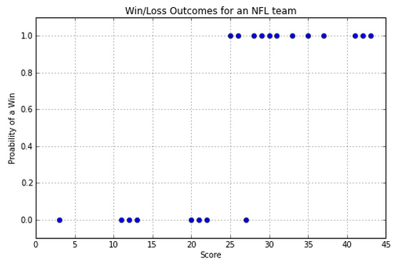
So, how do we predict whether we have a win or a loss if we are given a score? Note that we are going to be predicting values between 0 and 1. Close to 0 means we're sure it's in class 0, close to 1 means we're sure it's in class 1, and closer to 0.5 means we don't know.
Linear regression gets the general trend but it doesn't accurately represent the steplike behavior:
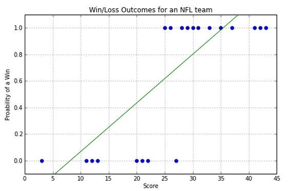
How would we use this model to estimate the class label (zero or one)?
Note mismatch between residual and "binarized" estimate.
So a line is not the best way to model this data. Luckily we know of a better curve.
Smooth change between outcomes with adjustable location and slope.
Smooth intermediate values model intermediate probabilities of class.
x = np.linspace(-10,10,100)

plt.figure(figsize=(8,2))
plt.plot(x,1/(1+np.exp(-1*x)), linewidth='1.7');
plt.plot(x,1/(1+np.exp(-2*x)), linewidth='1.7');
plt.plot(x,1/(1+np.exp(-1*(x-5))), linewidth='1.7');

plt.ylim(-0.001,1.01);
plt.legend((r'$\frac{1}{1+e^{-x}} = \sigma(x)$', r'$\frac{1}{1+e^{-2x}} = \sigma(2x)$', r'$\frac{1}{1+e^{-(x-5)}} = \sigma(x-5)$'), fontsize=14);
plt.grid();

Suppose we have a lot of data for something with two classes, such as their temperature relative to some baseline, and whether they have an infection.
For example $(x,y) =$ (-3.5, healthy), (+1.2, sick), (+2.05, healthy), ...
Our goal is to make a model to predict if someone is sick.
Define $x$ as the relative temperature. We can estimate the probability $p(x)$ if we have enough data, by using the measurements close to $x$, by binning them similar to a histogram.
$$ p(\text{Sick}) \approx \frac{\text{Number of measurements when patient is sick, and $x$ is in range $[x-\Delta,x+\Delta]$} }{\text{Number of total measurements when $x$ is in range $[x-\Delta,x+\Delta]$}} $$We can then estimate the odds and log-odds of this outcome.
Note that we can think of our estimated $p(\text{Sick}) $ like points sampled from a function. Logistic regression fits a model to these points.

The odds of an event $x_i$ happening is defined as
$$ \text{Odds} = \frac{\text{Probability of event happening}}{\text{Probability of event not happening}} = \frac{p(x_i)}{1-p(x_i)} $$If this is less than one, the odds are against you, for example.
Note that since $0 \le p \le 1$, the odds can range between zero and infinity.
The log-odds, known as the logit function, is the log of the odds function for an event,
$$ \text{logit}(p) = \log\frac{p(x_i)}{1-p(x_i)} $$The logit ranges between plus and minus infinity. Often handier to work with than probabilities.
Recall that the information is defined as $-\log(p)$ for an event. So the logit gives the information difference between the two possible outcomes, positive if the event is more likely to occur.
To fit: minimize $e^2 = \big( f( x;\beta_0, \beta_1) -y \big)^2$ to find optimal $\beta_0$ and $\beta_1$ ~ LMS Loss, a.k.a. L2, Least Squares
How might we fit this one?
We could theoretically fit a simple linear regression model to the logit of $p$,
$$ \operatorname{logit}(p(\text{Sick})) = \beta_0 + \beta^\top x, $$
Then the model for $p(\text{Sick})$ is given via the logistic function $$ p(x)=\frac{1}{1+e^{-(\beta_0+\beta^\top x)}}. $$
But we have to estimate $\operatorname{logit}(p(\text{Sick}))$ to do this
show_logistic_example()


So we get $P(y=1)+P(y=0)=1$, and at the mid point of the transition, we get $P(y=1)=P(y=0)=0.5$, like probabilities. This midpoint is called the decision boundary.
Note we can write this compactly as
\begin{align} "P(y|x)" &= P(y=1)^y P(y=0)^{1-y} \notag \\ &= P(y=1)^y (1-P(y=1))^{1-y} \notag \\ \end{align}This is the same as
$$ P(y|x) = \begin{cases} P(y=1|x) = \sigma(\beta_0 + \beta_1 x), \text{ if } y=1 \\ P(y=0|x) = 1-\sigma(\beta_0 + \beta_1 x), \text{ if } y=0 \\ \end{cases} $$The exponent $y$ is used to select the cases, since $y$ can only be zero or one.
Just choose the class with higher probability.
$$ \hat{c} = \begin{cases} 1, \text{ if } P(y = 1) > 0.5 \\ 0, \text{ else } \end{cases} $$Consider a general Bernoulli random variable measurement $y_i$ which has probability $p_i$ of taking value 1: $$ P(y_i\mid x_i;\beta_0,\beta_1) = p_i^{\,y_i}(1-p_i)^{1-y_i} = \begin{cases} p_i, & y_i=1 \\ 1-p_i, & y_i=0 \end{cases} $$
The likelihood function $L$ for an i.i.d. dataset of $n$ observations is $$ L(\beta_0,\beta_1) = \prod_{i=1}^{n} p_i^{y_i} (1 - p_i)^{1 - y_i} $$
we take the log to get $$ \log L(\beta_0,\beta_1) = \sum_{i=1}^{n} [y_i \log(p_i) + (1 - y_i) \log(1 - p_i)] $$
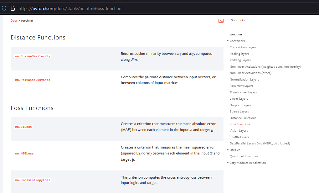
In machine learning, we use the closely-related Binary Cross-Entropy (BCE) loss $$ BCE = -\frac{1}{n}\sum_{i=1}^{n} [y_i \log(p_i) + (1 - y_i) \log(1 - p_i)] $$
Minimizing this maximizes the log-likelihood, since $BCE = -\frac{1}{n}\log L(\beta_0,\beta_1)$.
As $n \rightarrow \infty$, the average in the BCE becomes an expected value over the data. Write $q(x) = P_{\text{true}}(1 \mid x)$ for the true probability and $p(x) = P_{\text{model}}(1 \mid x) = \sigma(\beta_0 + \beta_1 x)$ for the model's. Since $\mathbb{E}[y \mid x] = q(x)$, $$ BCE \rightarrow \mathbb{E}_x\Big[-q(x)\log p(x) - \big(1-q(x)\big)\log\big(1-p(x)\big)\Big] = \mathbb{E}_x\Big[H\big(P_{\text{true}}(\cdot \mid x), P_{\text{model}}(\cdot \mid x)\big)\Big] $$ the cross-entropy between the true and model probabilities at each $x$, averaged over $x$.
At each $x$, the cross-entropy $f(p) = -q\log p - (1-q)\log(1-p)$ is smallest when the model probability equals the true one: $$ f'(p) = -\frac{q}{p} + \frac{1-q}{1-p} = \frac{p-q}{p(1-p)} = 0 \quad\Longrightarrow\quad p = q, \qquad f''(p) = \frac{q}{p^2} + \frac{1-q}{(1-p)^2} > 0 $$ So minimizing the BCE makes $P_{\text{model}}(1 \mid x)$ estimate $P_{\text{true}}(1 \mid x)$. If the true log-odds are not linear in $x$, it gives the sigmoid closest to $P_{\text{true}}$ in cross-entropy.
For a finite sample, setting the gradient of the BCE to zero gives $\sum_i (y_i - p_i) = 0$ and $\sum_i (y_i - p_i)\,x_i = 0$: the predicted probabilities add up to the observed number of 1s (observed = expected, lecture 06).
Recall $P_{\text{model}}$ is our sigmoid model, while the data represents the true distribution $P_{\text{true}}$, so we are optimizing to match our model to the data by minimizing the cross entropy between them
also we are dealing with an estimator, often called the empirical cross-entropy
$H(P_{\text{true}})$ is the entropy of the data. It does not depend on the model parameters $\beta_0, \beta_1$, so minimizing the cross-entropy (the BCE) also minimizes the KL divergence: the same $\beta_0, \beta_1$ minimize both.
The minimum values differ, though. The KL divergence reaches 0 when $P_{\text{model}} = P_{\text{true}}$, while the cross-entropy can only get down to $H(P_{\text{true}})$. That is why the BCE of even a perfect model stays above zero when the labels are uncertain.
In terms of the logit $z_i = \beta_0 + \beta_1 x_i$, where $p_i = \sigma(z_i)$.
Note $\log\sigma(z) = -\log(1+e^{-z})$ and $\log(1-\sigma(z)) = -z-\log(1+e^{-z})$
each term above simplifies to $y_i z_i - \log(1+e^{z_i})$, so
$$
BCE(\beta_0,\beta_1) = \frac{1}{n}\sum_{i=1}^{n} \Big[\log\big(1+e^{\beta_0+\beta_1 x_i}\big) - y_i(\beta_0+\beta_1 x_i)\Big]
$$
torch.nn.BCEWithLogitsLoss uses this form to avoid taking $\log 0$ when $p_i$ rounds to 0 or 1.
https://docs.pytorch.org/docs/stable/generated/torch.nn.BCEWithLogitsLoss.html
Contrast the one-dimensional case (one feature)
Contrast the two-dimensional case (two features)
What do binary labels look like in 1D versus 2D?
Hui & Belkin (ICLR 2021) "Evaluation of neural architectures trained with square loss vs cross-entropy in classification tasks" (https://arxiv.org/abs/2006.07322)
trained standard neural networks for NLP, speech and vision with square loss on the raw outputs against one-hot labels, instead of softmax cross-entropy
Counter-arguments:
Try using part of the BRFSS data to predict one variable from others.
Compare a logistic regression model using BCE loss to a linear model using MSE loss
Binary logistic regression makes the log-odds of one class against the other linear in the features: $$ \log\frac{p_i}{1-p_i} = \beta_0 + \beta_1 X_{i,1} + \dots + \beta_n X_{i,n} $$ With $K$ classes, let $p_{i,k}$ be the probability that observation $i$ is in class $k$. Pick one class, say $K$, as the baseline, and make the log-odds of each other class against it linear in the features: $$ \log\frac{p_{i,k}}{p_{i,K}} = z_{i,k} = \beta_{k,0} + \beta_{k,1} X_{i,1} + \dots + \beta_{k,n} X_{i,n}, \qquad k = 1, \dots, K-1 $$ Each class $k$ has its own coefficients $\beta_{k,0}, \dots, \beta_{k,n}$, so there are $(K-1)(n+1)$ in all. For $K = 2$ this is binary logistic regression.
In statistics this is a generalized linear model (GLM): a categorical response, a linear predictor $z_{i,k}$, and the baseline-category logit $\log(p_{i,k}/p_{i,K})$ as the link function. Linear regression (Gaussian response, identity link) and binary logistic regression (Bernoulli response, logit link) are GLMs too. Because the response is a one-hot vector, this one is strictly a multivariate GLM.
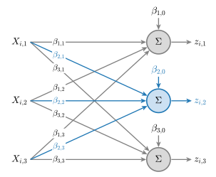
Exponentiating the log-odds gives $p_{i,k} = p_{i,K}\, e^{z_{i,k}}$ for $k = 1, \dots, K-1$. The probabilities sum to 1: $$ p_{i,K} + \sum_{l=1}^{K-1} p_{i,K}\, e^{z_{i,l}} = 1 \quad\Longrightarrow\quad p_{i,K} = \frac{1}{1 + \sum_{l=1}^{K-1} e^{z_{i,l}}} $$ so $$ p_{i,k} = \frac{e^{z_{i,k}}}{1 + \sum_{l=1}^{K-1} e^{z_{i,l}}}, \qquad k = 1, \dots, K-1 $$ Set the baseline's logit to $z_{i,K} = 0$, so $e^{z_{i,K}} = 1$. Then every class, including the baseline, has the same form, the softmax: $$ p_{i,k} = \frac{e^{z_{i,k}}}{\sum_{l=1}^{K} e^{z_{i,l}}}, \qquad k = 1, \dots, K $$ For $K = 2$, $p_{i,1} = \dfrac{e^{z_{i,1}}}{1 + e^{z_{i,1}}} = \sigma(z_{i,1})$, the sigmoid.
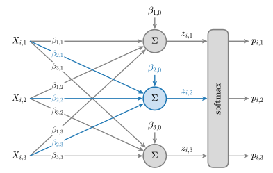
The diagram has a logit for every class, $z_{i,k} = \beta_{k,0} + \beta_{k,1} X_{i,1} + \dots + \beta_{k,n} X_{i,n}$ for $k = 1, \dots, K$. Adding the same constants $c_0, c_1, \dots, c_n$ to every class's coefficients adds the same $c_i = c_0 + c_1 X_{i,1} + \dots + c_n X_{i,n}$ to every logit, and the softmax does not change: $$ \frac{e^{z_{i,k} + c_i}}{\sum_{l=1}^{K} e^{z_{i,l} + c_i}} = \frac{e^{z_{i,k}}}{\sum_{l=1}^{K} e^{z_{i,l}}} $$ Only differences of logits matter, $z_{i,k} - z_{i,l} = \log(p_{i,k}/p_{i,l})$, so one class's worth of coefficients is redundant.
The multinomial logit model removes the redundancy with a baseline, $z_{i,K} = 0$:
Deep learning keeps the redundancy:
For $K = 2$, deep learning also uses the baseline form: one logit and a sigmoid.
Encode the label of observation $i$ as one-hot: $y_{i,k} = 1$ if observation $i$ is in class $k$, and $0$ otherwise. One observation has a categorical distribution, which generalizes the Bernoulli: $$ P(y_i \mid X_{i,1}, \dots, X_{i,n}; \beta) = \prod_{k=1}^{K} p_{i,k}^{\,y_{i,k}} $$ The exponents select the factor for the observed class. The likelihood for $m$ independent observations is $$ L(\beta) = \prod_{i=1}^{m} \prod_{k=1}^{K} p_{i,k}^{\,y_{i,k}} $$ and we take the log to get $$ \log L(\beta) = \sum_{i=1}^{m} \sum_{k=1}^{K} y_{i,k} \log p_{i,k} $$
As for the BCE, take negative average:
$$ CE(\beta) = -\frac{1}{m} \log L(\beta) = -\frac{1}{m} \sum_{i=1}^{m} \sum_{k=1}^{K} y_{i,k} \log p_{i,k} $$Minimizing this maximizes the log-likelihood. For $K = 2$, with $y_{i,1} = y_i$, $y_{i,2} = 1 - y_i$ and $p_{i,1} = p_i$, it is the BCE.
As with binary logistic regression there is no closed-form solution, so the $\beta$s are found numerically.
Source: ISLR/ISLP §4.3.5.
A GLM has three parts:
$^*$ canonical link, up to a constant factor. $\Phi$ is the standard Normal CDF, and the $\theta_k$ are cutpoints between the ordered classes.
Smooth approximation to argmax. Outputs a probability distribution over classes.
Given logits ( x = [2, 1, 0] ):
$$ \text{softmax}(x_i) = \frac{e^{x_i}}{\sum_{j} e^{x_j}} $$Compute the denominator:
$$ \sum_{j} e^{x_j} = e^2 + e^1 + e^0 = 7.389 + 2.718 + 1 = 11.107 $$Thus:
$$ \text{softmax}(x) = \left[ \frac{7.389}{11.107}, \frac{2.718}{11.107}, \frac{1.000}{11.107} \right] = [0.665, 0.245, 0.090] $$Softmax acts as a continuous relaxation of the one-hot (argmax) operation. As one logit dominates, the output converges to the corresponding basis vector; for finite $a$, it produces a smooth, differentiable approximation.
If $x \in \mathbb{R}^n$ is sparse with a single nonzero element at index $k$, then
$$ x_i = \begin{cases} a, & i = k \\ 0, & i \neq k \end{cases} $$The softmax is
$$ p_i = \frac{e^{x_i}}{\sum_{j=1}^n e^{x_j}} = \frac{e^{x_i}}{e^{a} + (n-1)e^{0}} = \frac{e^{x_i}}{e^{a} + n - 1}. $$Hence,
$$ p_k = \frac{e^{a}}{e^{a} + n - 1}, \qquad p_{i \ne k} = \frac{1}{e^{a} + n - 1}. $$As $a \to \infty$:
$$ p_k \to 1, \qquad p_{i \ne k} \to 0, $$so
$$ \lim_{a \to \infty} \text{softmax}(x) = e_k, $$where $e_k$ is the $k$-th standard basis vector.
# Softmax: distribution for logits [x, 0, -x]

def softmax(logits, axis=-1):
    z = logits - np.max(logits, axis=axis, keepdims=True)
    expz = np.exp(z)
    return expz / np.sum(expz, axis=axis, keepdims=True)

x = np.linspace(-8, 8, 400)
logits = np.stack([x, np.zeros_like(x), -x], axis=1)

plt.figure()
plt.plot(x, logits[:, 0], label='class 0')
plt.plot(x, logits[:, 1], label='class 1')
plt.plot(x, logits[:, 2], label='class 2')

plt.title('Logit values vs x')
#plt.xlabel('x')
plt.ylabel('logit')
plt.grid(True)
plt.legend()
plt.show()


probs = softmax(logits, axis=1)
plt.figure()
plt.plot(x, probs[:, 0], label='p(class 0)')
plt.plot(x, probs[:, 1], label='p(class 1)')
plt.plot(x, probs[:, 2], label='p(class 2)')
plt.plot(x, np.sum(probs,1), '--', label='sum over probs')

plt.title('Softmax probabilities vs x')
plt.xlabel('x')
plt.ylabel('probability')
plt.grid(True)
plt.legend()
plt.show()


Binary softmax:
$$ p_1 = \frac{e^{z_1}}{e^{z_1} + e^{z_2}}, \qquad p_2 = \frac{e^{z_2}}{e^{z_1} + e^{z_2}}. $$Fix $z_2 = 0$ and rename $z_1 = z$:
$$ p_1 = \frac{e^{z}}{e^{z} + 1} = \sigma(z), \qquad p_2 = 1 - \sigma(z). $$Thus the sigmoid is a 2-class softmax.
Temperature $T>0$ controls sharpness:
$$
\text{softmax}_T(x_i) =
\frac{e^{x_i / T}}{\sum_j e^{x_j / T}}.
$$
As $T \to 0$: one-hot.
As $T \to \infty$: uniform.
With $K$ classes, encode the label of observation $i$ as a one-hot vector $y_i = (y_{i,1}, \dots, y_{i,K})$, where $y_{i,k} = 1$ if observation $i$ is in class $k$ and $0$ otherwise, so $y_i = e_k$, the $k$-th standard basis vector.
The Bernoulli distribution generalizes to the categorical distribution, with class probabilities $p_k \ge 0$, $\sum_{k=1}^{K} p_k = 1$: $$ P(y_i) = \prod_{k=1}^{K} p_k^{\,y_{i,k}} $$ As in the Bernoulli case, the exponents select the factor for the observed class. For $K = 2$, with $y_{i,1} = y_i$ and $y_{i,2} = 1 - y_i$, this is $p^{\,y_i}(1-p)^{1-y_i}$.
The question is how the $p_k$ should depend on the features $x = (x_1, \dots, x_n)$.
Bayes' rule gives the class probabilities in terms of the class-conditional densities $P(x \mid k)$ and the class priors $P(k)$: $$ P(k \mid x) = \frac{P(x \mid k)\,P(k)}{\sum_{l=1}^{K} P(x \mid l)\,P(l)} $$ Write each term as an exponential, $P(x \mid k)\,P(k) = e^{z_k}$, so $z_k = \log P(x \mid k) + \log P(k)$. Then $$ P(k \mid x) = \frac{e^{z_k}}{\sum_{l=1}^{K} e^{z_l}} = \operatorname{softmax}(z)_k $$ Nothing has been assumed yet: softmax is Bayes' rule written with log joint probabilities as the logits. A constant added to every $z_k$ cancels, so only differences of logits matter.
For $K = 2$, dividing through by $e^{z_1}$, $$ P(1 \mid x) = \frac{1}{1 + e^{-(z_1 - z_2)}} = \sigma(z_1 - z_2), \qquad z_1 - z_2 = \log\frac{P(1 \mid x)}{P(2 \mid x)} $$ so the sigmoid's input is the log-odds, as in the binary case.
To go further, choose the class-conditional densities. If the features in class $k$ are Gaussian with mean $\mu_k$ and a covariance $\Sigma$ shared by all classes (the multivariate Gaussian of lecture 02), then $$ z_k = -\tfrac12 (x - \mu_k)^T \Sigma^{-1} (x - \mu_k) + \log P(k) + \text{const} $$ Expanding, the term $-\tfrac12 x^T \Sigma^{-1} x$ and the constant are the same for every class, so they cancel in the softmax and can be dropped. What remains is linear in $x$: $$ z_k = \beta_{k,0} + \beta_{k,1} x_1 + \dots + \beta_{k,n} x_n, \qquad \beta_{k,j} = (\Sigma^{-1} \mu_k)_j, \qquad \beta_{k,0} = -\tfrac12 \mu_k^T \Sigma^{-1} \mu_k + \log P(k) $$ This is linear discriminant analysis (LDA), a generative model: estimate $\mu_k$, $\Sigma$ and $P(k)$ from the data, and the $\beta$s follow.
Multinomial logistic regression is the discriminative version. It keeps the softmax of linear logits but fits the $\beta_{k,j}$ directly to the labels, without assuming Gaussian features. For observation $i$ with features $X_{i,1}, \dots, X_{i,n}$: $$ z_{i,k} = \beta_{k,0} + \beta_{k,1} X_{i,1} + \dots + \beta_{k,n} X_{i,n}, \qquad p_{i,k} = \frac{e^{z_{i,k}}}{\sum_{l=1}^{K} e^{z_{i,l}}} $$ Since only differences of logits matter, one class's $\beta$s can be fixed at 0. For $K = 2$ this leaves one set of $\beta$s, and the model is logistic regression.
By the same argument as for the BCE, as $m \to \infty$ the average over observations becomes an expected value over the data: $$ CE \to \mathbb{E}_x\Big[-\sum_{k=1}^{K} P_{\text{true}}(k \mid x) \log P_{\text{model}}(k \mid x)\Big] = \mathbb{E}_x\Big[H\big(P_{\text{true}}(\cdot \mid x), P_{\text{model}}(\cdot \mid x)\big)\Big] $$ and since $H(P_{\text{true}})$ does not depend on $\beta$, minimizing the cross-entropy also minimizes $D_{KL}(P_{\text{true}} \parallel P_{\text{model}})$.
In terms of the logits, the loss for observation $i$ is
$$
-\log p_{i,c_i} = -z_{i,c_i} + \log \sum_{l=1}^{K} e^{z_{i,l}}
$$
torch.nn.CrossEntropyLoss takes the logits $z_{i,k}$ and the class indices $c_i$ and computes this with a stable log-sum-exp, so a model trained with it should output logits, with no softmax layer.
Sources: PRML §4.2 and §4.3.4; ISLR/ISLP §4.3.5 and §4.4. See References at the top.
LLMs produce a probability distribution over the next token by outputting a value which can be interpreted as a logit for every token in the vocabulary.
The logits $z \in \mathbb{R}^V$ are unconstrained real numbers. They are converted into probabilities with the softmax:
$$ p(\text{token } i \mid \text{context}) = \frac{e^{z_i}}{\sum_{j=1}^V e^{z_j}}. $$Logits encode relative token preference because
$$ \log \frac{p(i)}{p(j)} = z_i - z_j. $$Training adjusts model parameters so that these softmax probabilities match the training distribution (cross-entropy).
Decoding methods (sampling, greedy, temperature scaling) operate directly on the logits.
The simplest measure is accuracy. This is the number of correct predictions over the total number of predictions. It's the percent you predicted correctly. In sklearn, this is what the score method calculates.
Accuracy is a good first glance measure, but it has shortcomings.
If the classes are unbalanced, accuracy will not measure how well you did at predicting. Say you are trying to predict whether or not an email is spam. Only 2% of emails are in fact spam emails. You could get 98% accuracy by always predicting not spam. This is a great accuracy but a horrible model!
What additional measurements might we do to check for such failures?
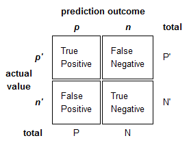
We can get a better picture our model by looking at the confusion matrix. We get the following four metrics:
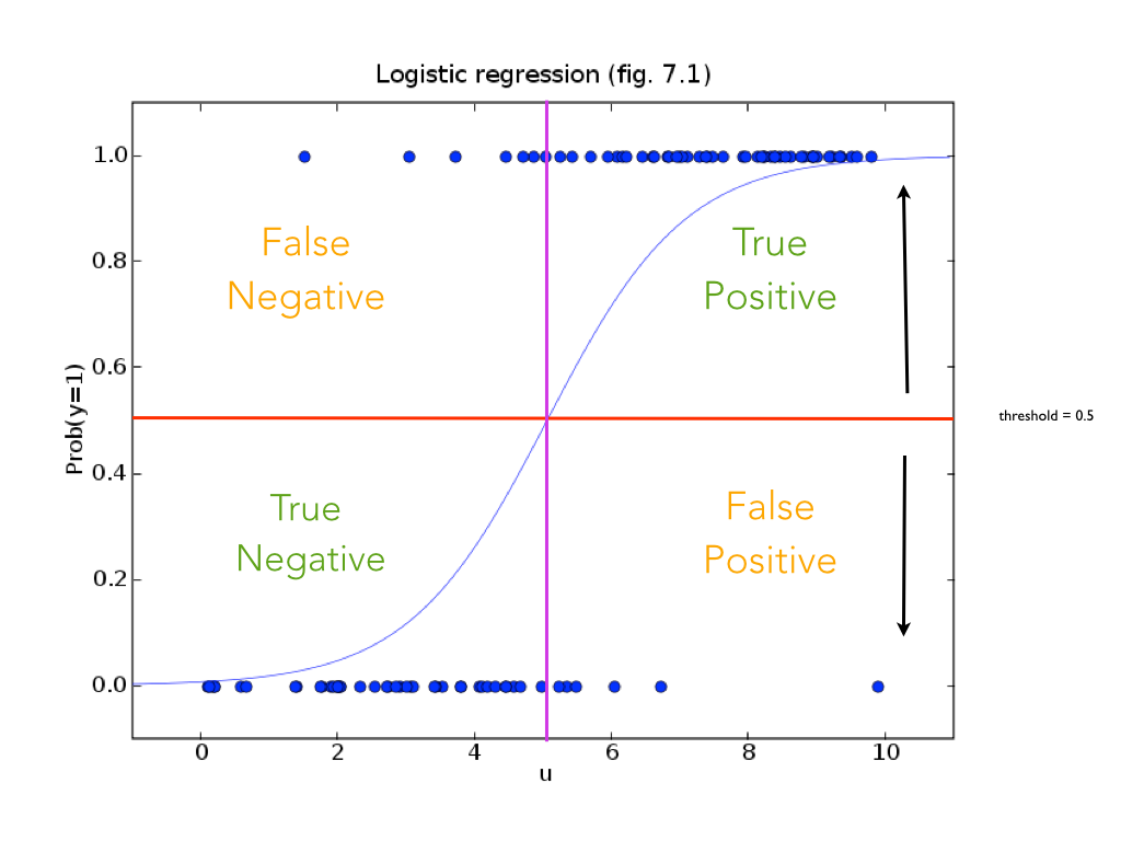
Note what happens as you move the decision threshold.
  Precison = TP / (TP + FP)
           = TP / (predicted yes) = fraction of correct 1's
Sensitivity = TP / (TP + FN)
= TP / (actual yes) F1 = 2 / (1/Precision + 1/Sensitivity)
= 2 * Precision * Recall / (Precision + Sensitivity)
= 2TP / (2TP + FN + FP)Youden's Index (sometimes called J statistic) is similar to the F1 score in that it is a single number that describes the performance of a classifier.
$$J = Sensitivity + Specificity - 1$$$$where$$$$Sensitivity = \frac{TP}{TP + FN}$$$$Specificity = \frac{TN}{TN + FP}$$The J statistic ranges from -1 to 1 (negative is worse than random):
It can be thought of as an improvement on the F1 score since it takes into account all of the cells in a confusion matrix. It can also be used to find the optimal threshold for a given ROC curve.
Suppose that you're using linear regression to predict 0-1 labels. You train your model and on the test data you get the following results. Calculate TP, FP, TN, FN
labels = [0,0,0,0,0,1,1,1,1,1]
predictions = [-0.8, -0.4, 0.0, 0.4, 0.8, 0.2, 0.6, 1.0, 1.4, 1.8]
threshold = .5

#calculate TP, FP, TN, FN
Now suppose
How much does your predictor cost with a threshold value of 0.5?
Generate costs for threshold values of 0.0, 0.25, 0.5, 0.75 and 1.0.
Which one yields the minimum cost?
Explain any shift in the threshold from 0.5.
Very popular way to visualize classifier performance. (http://en.wikipedia.org/wiki/Receiver_operating_characteristic)
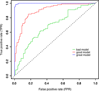
ROC curve = true positive rate (TPR) versus false positive rate (FPR).
\begin{align} \text{True Positive Rate} &= TPR = \frac{\text{number of true positives}}{\text{number of actual positives}} \\ \text{False Positive Rate} &= FPR = \frac{\text{number of false positives}}{\text{number of actual negatives}} \\ \end{align}What are the rates for random guessing?
import numpy as np
import matplotlib.pyplot as plt
%matplotlib inline

labels = [0,0,0,0,0,1,1,1,1,1]
predictions = [-0.8, -0.4, 0.0, 0.4, 0.8, 0.2, 0.6, 1.0, 1.4, 1.8]