Mathematical Methods for Data Science
Keith Dillon
Spring 2020
Topic 2: "Classical" Linear Algebra Software
This topic:
- BLAS, LAPACK, Eigen
- Overview of major python packages
- Structured and Sparse Linear Algebra
- Numpy basics
Reading: the internet
What is "Classical" Linear Algebra software?
- A term I just invented
- Generally single CPU, RAM-limited implementations of well-known algorithms (e.g. Golub & Van Loan "Matrix Computations")
- ...and higher-level packages based on these algorithms, inheriting the limitations
- Large-scale (more than 10k variable or so) only possible via sparse linear algebra algorithms
- Leading parallel tool is SIMD (single instruction multiple data) via math co-processors.
- More parralelism at top-level rather than bottom ("workers" running seperate processes on separate CPU's)
- current growth is in rewriting basic algorithms for
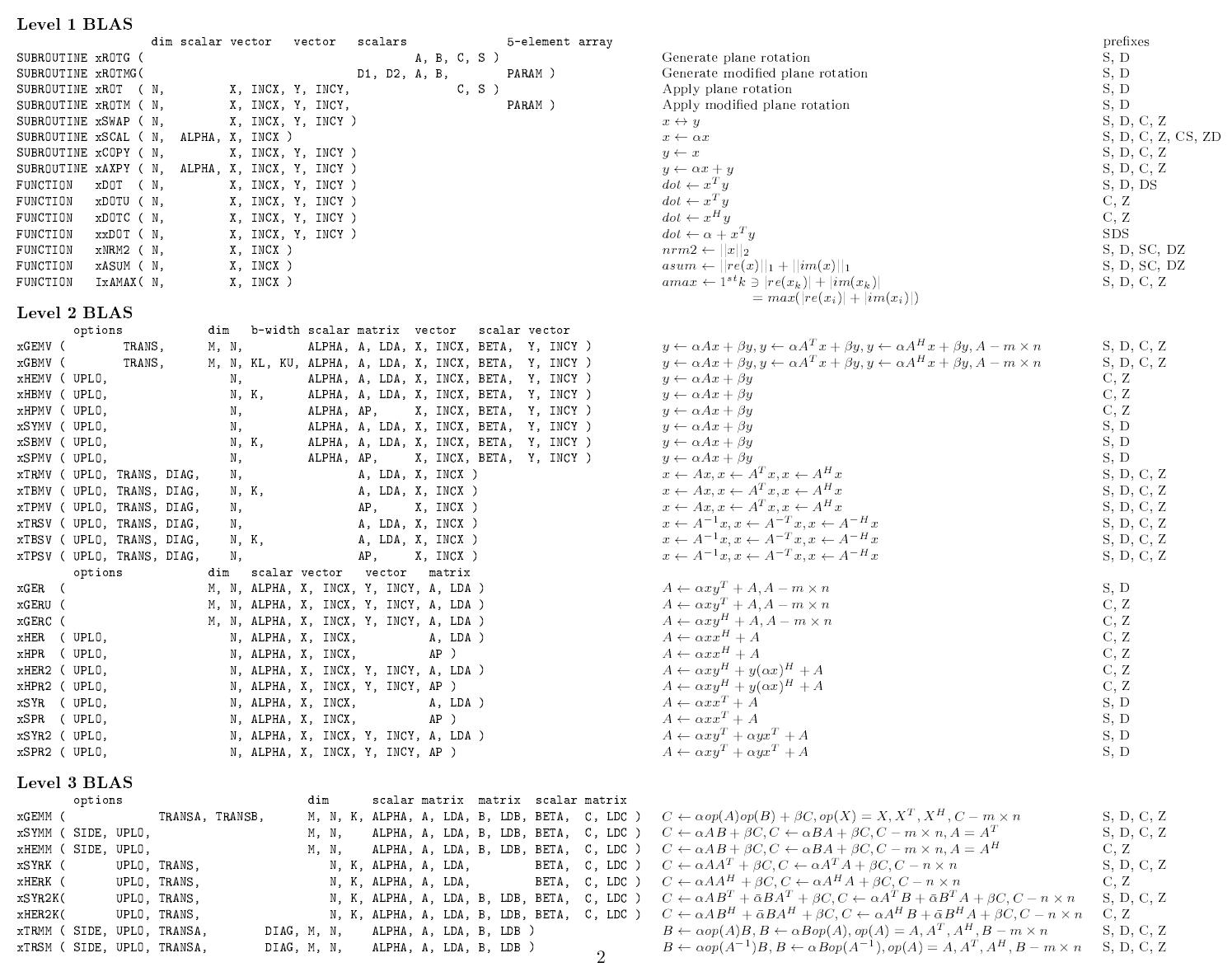
I. BLAS BLAS BLAS
BLAS = Basic Linear Algebra Subroutines
Efficient algorithms for matrix algebra
- scaling, multiplying. "Level 1,2,3 functions"
- single and double precision, real and complex numbers
- generally don't take advantage of multiple threads or CPU's by chip maker
- Are often optimized for complex instructions however, e.g. SIMD
- Originally FORTRAN - one-based, columns first, like matlab
- various implementations, including parallelizable versions, C/C++ CUDA,
- http://www.netlib.org/blas/
BLAS Levels 1,2,3 ~ $O(n), O(n^2), O(n^3)$
import scipy.linalg.blas as blas

dir(blas)
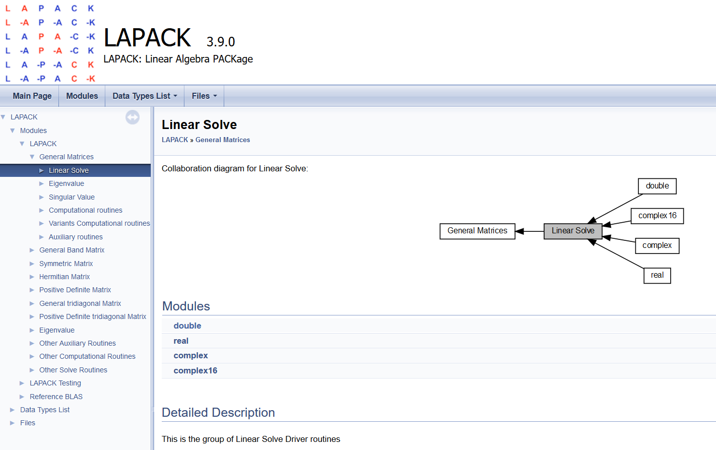
LAPACK = Linear Algebra Package
- Fortran, Uses BLAS as backend (can choose different implementations)
- http://www.netlib.org/lapack/
- https://github.com/Reference-LAPACK/lapack
- systems of simultaneous linear equations
- least-squares solutions of linear systems of equations
- eigenvalue problems
- singular value problems.
- associated matrix factorizations (LU, Cholesky, QR, SVD, Schur, generalized Schur)
- related computations such as reordering of the Schur factorizations and estimating condition numbers.
- Dense and banded matrices are handled, but not general sparse matrices.
- real and complex matrices
- both single and double precision.
- Matlab, and the Python tools we will use were essentially built on this
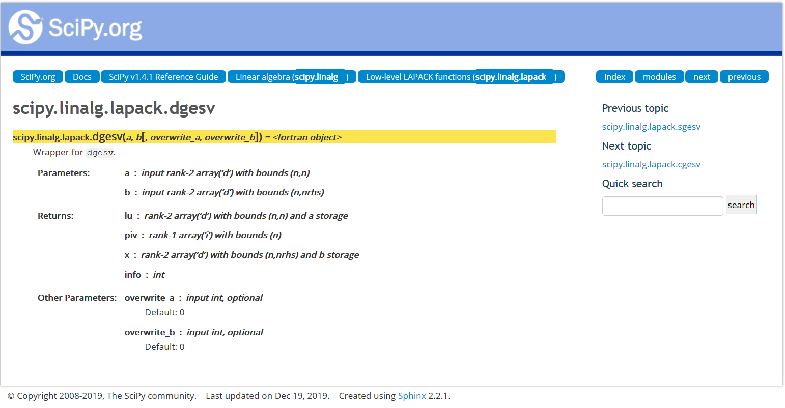
import scipy.linalg.lapack as lapack

dir(lapack)
C++ API
Scipy wrapper API
Eigen
- https://eigen.tuxfamily.org/dox/
- Written in C++
- Used for linear algebra in Tensorflow (single CPU variant probably)
- Low and high-level (e.g. matrix decompositions) linear algebra functions
- Sparse linear algebra
...name can be annoyingly google-proof however
Take-home message
Much (most) code you get for free, or even pay for, that implements mathematical algorithms may be of limited value.
Linear algebra, however, is "solved", in terms of numerical programming.
Your main concern is to find an implementation that fits for your application. E.g. parallel, or sparse, or optimized for a particular CPU.
Lab: Import and directly use packages in Python
- BLAS - compute a dot product of two random vectors
- LAPACK - solve a random linear system
II. Overview of leading Python math tools
Leading Python tools:
Jupyter - "notebooks" for inline code + LaTex math + markup, etc.
NumPy - low-level array & matrix handling and algorithms
SciPy - higher level numerical algorithms (still fairly basic)
Matplotlib - matlab-style plotting & image display
SkLearn - (Scikit-learn) Machine Learning library
NumPy
- Numerical algorithm toolbox
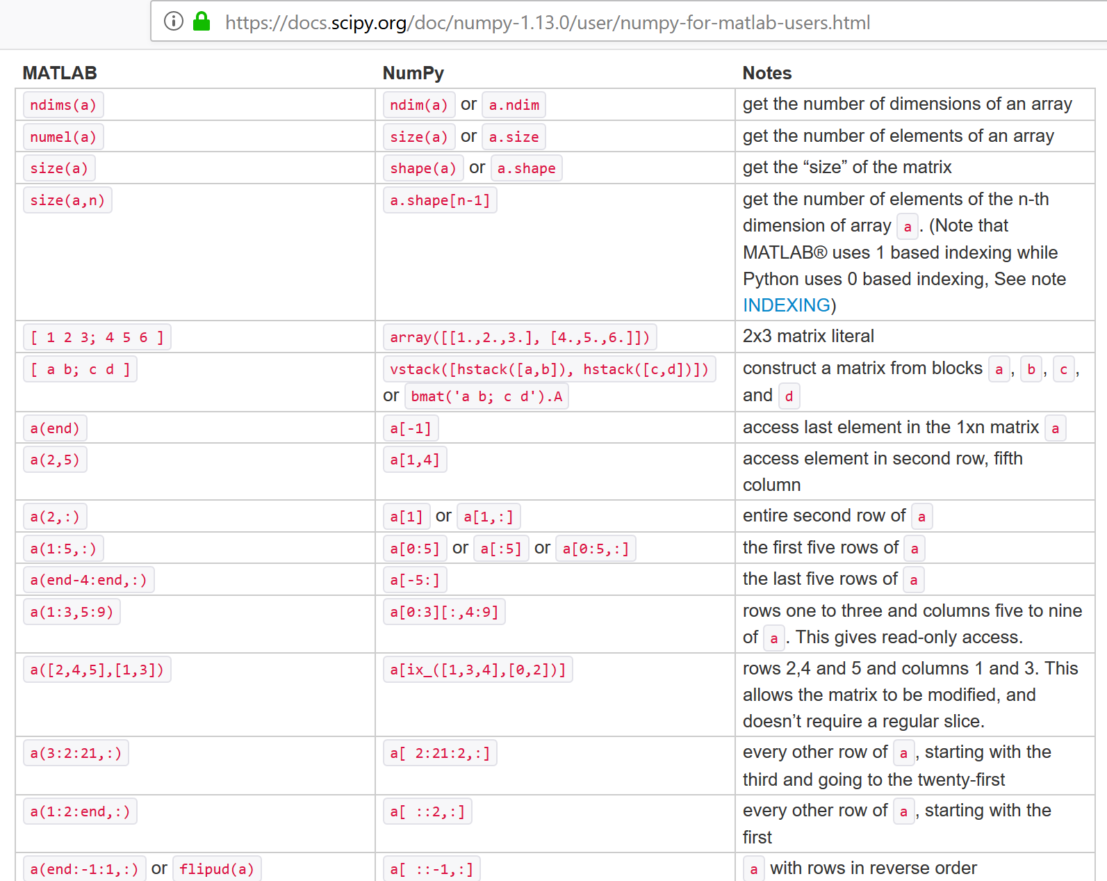
- Similar to Matlab but Many key differences, such as zero-based indexing (like C) instead of one-based (like math texts).
- Uses BLAS/LAPACK typically
- NumPy Arrays - special data structure which allows direct and efficient linear algebra manipulations (basically a list with added functionality).
import numpy as np

x = np.array([2,0,1,8])

print(x)
Fast Numerical Mathematics
l = range(1234)
%timeit [i ** 2 for i in l]
import numpy as np
a = np.arange(1234)
%timeit a ** 2
NumPy for Matlab Users
help(np.array)
Will cover more later, but first a quick intro to some other packages.
SciPy
Implements higher-level scientific algorithms using NumPy. Examples:
- Integration (scipy.integrate)
- Optimization (scipy.optimize)
- Interpolation (scipy.interpolate)
- Signal Processing (scipy.signal)
- Linear Algebra (scipy.linalg)
- Statistics (scipy.stats)
- File IO (scipy.io)
Also uses BLAS/LAPACK
import scipy
dir(scipy)
Matplotlib
Tutorial from: https://github.com/amueller/scipy-2017-sklearn/blob/master/notebooks/02.Scientific_Computing_Tools_in_Python.ipynb
Another important part of machine learning is the visualization of data. The most common
tool for this in Python is matplotlib. It is an extremely flexible package, and
we will go over some basics here.
Jupyter has built-in "magic functions", the "matoplotlib inline" mode, which will draw the plots directly inside the notebook. Should be on by default.
%matplotlib inline

import matplotlib.pyplot as plt

# Plotting a line
x = np.linspace(0, 10, 100)
plt.plot(x, np.sin(x));

# Scatter-plot points
x = np.random.normal(size=500)
y = np.random.normal(size=500)
plt.scatter(x, y);

# Showing images using imshow
# - note that origin is at the top-left by default!

#x = np.linspace(1, 12, 100)
#y = x[:, np.newaxis]
#im = y * np.sin(x) * np.cos(y)
im = np.array([[1, 2, 3],[4,5,6],[6,7,8]])
import matplotlib.pyplot as plt

plt.imshow(im);
plt.colorbar();
plt.xlabel('x')
plt.ylabel('y')
plt.show();

# Contour plots
# - note that origin here is at the bottom-left by default!
plt.contour(im);

# 3D plotting
from mpl_toolkits.mplot3d import Axes3D
ax = plt.axes(projection='3d')
xgrid, ygrid = np.meshgrid(x, y.ravel())
ax.plot_surface(xgrid, ygrid, im, cmap=plt.cm.viridis, cstride=2, rstride=2, linewidth=0);

There are many more plot types available. See matplotlib gallery.
Test these examples: copy the Source Code
link, and put it in a notebook using the %load magic.
For example:
# %load http://matplotlib.org/mpl_examples/pylab_examples/ellipse_collection.py
SkLearn
- Many Machine Learning functions.
- Couple dozen core developers + hundreds of other contributors.
- 2011 tutorial has over 10,000 citations.
"Scikit-learn: Machine Learning in Python", Fabian Pedregosa, Gaël Varoquaux, Alexandre Gramfort, Vincent Michel, Bertrand Thirion, Olivier Grisel, Mathieu Blondel, Peter Prettenhofer, Ron Weiss, Vincent Dubourg, Jake Vanderplas, Alexandre Passos, David Cournapeau, Matthieu Brucher, Matthieu Perrot, Édouard Duchesnay; 12(Oct):2825−2830, 2011
Considered leading Machine Learning toolbox. Was getting discarded as field switched from sinlge CPU to multicore, but appears to be making comeback with parallel upgrades
import sklearn as sk

dir(sk)
Machine Learning Framework using Sklearn
Given training data $(\mathbf x_{(i)},y_i)$ for $i=1,...,m$ --> lists of samples $\verb|X|$ and labels $\verb|y|$
Choose a model $f(\cdot)$ where we want to make $f(\mathbf x_{(i)})\approx y_i$ (for all $i$) --> choose sklearn estimator to use
Define a loss function $L(f(\mathbf x), y)$ to minimize by changing $f(\cdot)$ ...by adjusting the weights --> default choises for estimators, sometimes multiple options
The Sklearn API
sklearn has an Object Oriented interface
Most models/transforms/objects in sklearn are Estimator objects
class Estimator(object):

    def fit(self, X, y=None):
        """Fit model to data X (and y)"""
        self.some_attribute = self.some_fitting_method(X, y)
        return self

    def predict(self, X_test):
        """Make prediction based on passed features"""
        pred = self.make_prediction(X_test)
        return pred

model = Estimator()
The Estimator class defines a fit() method as well as a predict() method. For an instance of an Estimator stored in a variable model:
model.fit: fits the model with the passed in training data. For supervised models, it also accepts a second argumentythat corresponds to the labels (model.fit(X, y). For unsupervised models, there are no labels so you only need to pass in the feature matrix (model.fit(X))Since the interface is very OO, the instance itself stores the results of the
fitinternally. And as such you must alwaysfit()before youpredict()on the same object.model.predict: predicts new labels for any new datapoints passed in (model.predict(X_test)) and returns an array equal in length to the number of rows of what is passed in containing the predicted labels.
Types of subclass of estimator:
- Supervised
- Unsupervised
- Feature Processing
Supervised
Supervised estimators in addition to the above methods typically also have:
model.predict_proba: For classifiers that have a notion of probability (or some measure of confidence in a prediction) this method returns those "probabilities". The label with the highest probability is what is returned by themodel.predict()` mehod from above.model.score: For both classification and regression models, this method returns some measure of validation of the model (which is configurable). For example, in regression the default is typically R^2 and classification it is accuracy.
Unsupervised - Transformer interface
Some estimators in the library implement this.
Unsupervised in this case refers to any method that does not need labels, including unsupervised classifiers, preprocessing (like tf-idf), dimensionality reduction, etc.
The transformer interface usually defines two additional methods:
model.transform: Given an unsupervised model, transform the input into a new basis (or feature space). This accepts on argument (usually a feature matrix) and returns a matrix of the input transformed. Note: You need tofit()the model before you transform it.model.fit_transform: For some models you may not need tofit()andtransform()separately. In these cases it is more convenient to do both at the same time.
X = [[0], [1], [2], [3]]
y = [0, 0, 1, 1]
from sklearn.neighbors import KNeighborsClassifier
neigh = KNeighborsClassifier(n_neighbors=3)
neigh.fit(X, y)
print(neigh.predict([[1.1]]))
print(neigh.predict_proba([[0.9]]))
III. Structured and Sparse Matrices
Motivation
If you know your matric has particular structure, you can take advantage of this to greatly reduce computations and/or storage
Examples:
- Diagonal matrix
- Banded matrix
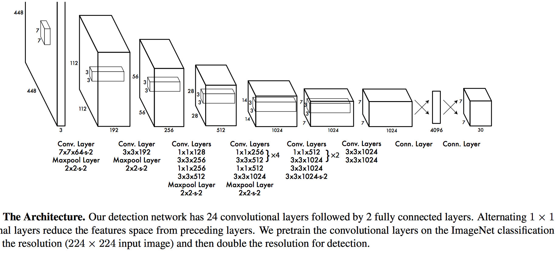
- Toeplitz (or circulant) matrix --> convolutional neural nets
- Sparse matrix
- Kronecker product
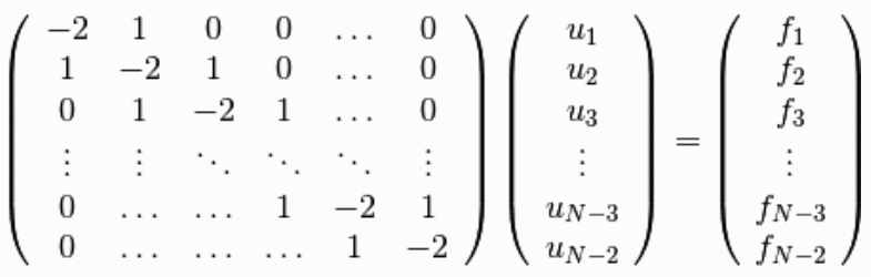
Structured matrix examples
How would you efficiently store these?
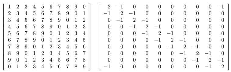
How might you efficiently multiple by a vector?
Examples
- Sparse structured matrices for which we don't have a specialized implementation
- Matrices describing sparse networks
scipy.sparse
SciPy 2-D sparse matrix package for numeric data.
https://docs.scipy.org/doc/scipy/reference/generated/scipy.sparse.csr_matrix.html
Sparse matrix types:
- bsr_matrix - Block Sparse Row matrix
- coo_matrix = A sparse matrix in COOrdinate format.
- csc_matrix - Compressed Sparse Column matrix
- csr_matrix - Compressed Sparse Row matrix
- dia_matrix - Sparse matrix with DIAgonal storage
- dok_matrix - Dictionary Of Keys based sparse matrix.
- lil_matrix - Row-based linked list sparse matrix
Different formats will be faster or slower for different tasks. Read API.
Compressed Sparse Row (CSR) Format
Stores list of values, list of column indices, and value-list indices for values that start each row
Also known as Compressed Row Storage CRS
from scipy.sparse import csr_matrix

indptr = np.array([0, 2, 3, 6])
indices = np.array([0, 2, 2, 0, 1, 2])
data = np.array([1, 2, 3, 4, 5, 6])
csr_matrix((data, indices, indptr), shape=(3, 3)).toarray()
# can also define with simple indices

row = np.array([0, 0, 1, 2, 2, 2])
col = np.array([0, 2, 2, 0, 1, 2])
data = np.array([1, 2, 3, 4, 5, 6])
csr_matrix((data, (row, col)), shape=(3, 3)).toarray()
Sparse solvers
- High-level algorithms that convert operations into BLAS calculations
- More limited implementations - sometimes no one yet happened to adapt a sparse solver to your particular problem
Exercise
Create two random matrices then make them sparse by zeroing out most elements (e.g. $\verb|A[A<0.99]=0|$)
Compare speed of matrix multiplication for different sparse formats
Recap
- Mathematical software is implemented hierarchically
- BLAS = Lowest level(s), implemented on particular hardware, e.g. for SIMD processors
- Higher level functions (solvers and decompositions) calls BLAS to implement internal computations
- Structured and Sparse matrix libraries also call BLAS typically (convert large sparse problems to small dense problems)
- Modern alternatives also can utilize BLAS/LAPACK backend and also suppot hardware-specific replacements (e.g. CUDA)
IV. NumPy Basics
NumPy Arrays for Vectors
x = np.array([2,0,1,8])

x
NumPy arrays are zero-based like Python lists, but linear algebra writings are typically one-based.
print(x[0],x[3])
What is a "Tensor"? (Computer Science version)
Behind the scenes it's just another list of numbers with some extra info regarding dimensions
Ndarray
https://docs.scipy.org/doc/numpy-1.13.0/reference/arrays.ndarray.html
A $d$-dimensional data structure, containing $n_1\times n_2 \times ... \times n_d$ numbers
np.random.rand(3)
np.random.rand(3,2) # note not a tuple (unlike many other numpy functions)
np.random.rand(3,2,4)
- A list of length 3,
- each of those 3 elements is a list of length 2
- each of those 2 elements is a list of length 4
T = np.random.rand(3,2,4,3,2)
T.shape
T.ndim
$\verb|numpy.linalg|$
- Use BLAS and LAPACK to provide efficient low level implementations of standard linear algebra algorithms.
- Those libraries may be provided by NumPy itself using C versions of a subset of their reference implementations
- When possible, highly optimized libraries that take advantage of specialized processor functionality are preferred.
- Examples of such libraries are OpenBLAS, MKL (TM), and ATLAS.
https://docs.scipy.org/doc/numpy/reference/routines.linalg.html
Matrix and vector products
- dot(a, b[, out]) Dot product of two arrays.
- linalg.multi_dot(arrays) Compute the dot product of two or more arrays in a single function call, while automatically selecting the fastest evaluation order.
- vdot(a, b) Return the dot product of two vectors.
- inner(a, b) Inner product of two arrays.
- outer(a, b[, out]) Compute the outer product of two vectors.
- matmul(x1, x2, /[, out, casting, order, …]) Matrix product of two arrays.
- tensordot(a, b[, axes]) Compute tensor dot product along specified axes.
- einsum(subscripts, *operands[, out, dtype, …]) Evaluates the Einstein summation convention on the operands.
- einsum_path(subscripts, *operands[, optimize]) Evaluates the lowest cost contraction order for an einsum expression by considering the creation of intermediate arrays.
- linalg.matrix_power(a, n) Raise a square matrix to the (integer) power n.
- kron(a, b) Kronecker product of two arrays.
Decompositions
- linalg.cholesky(a) Cholesky decomposition.
- linalg.qr(a[, mode]) Compute the qr factorization of a matrix.
- linalg.svd(a[, full_matrices, compute_uv, …]) Singular Value Decomposition.
Matrix eigenvalues¶¶
- linalg.eig(a) Compute the eigenvalues and right eigenvectors of a square array.
- linalg.eigh(a[, UPLO]) Return the eigenvalues and eigenvectors of a complex Hermitian (conjugate symmetric) or a real symmetric matrix.
- linalg.eigvals(a) Compute the eigenvalues of a general matrix.
- linalg.eigvalsh(a[, UPLO]) Compute the eigenvalues of a complex Hermitian or real symmetric matrix.
Norms and other numbers
- linalg.norm(x[, ord, axis, keepdims]) Matrix or vector norm.
- linalg.cond(x[, p]) Compute the condition number of a matrix.
- linalg.det(a) Compute the determinant of an array.
- linalg.matrix_rank(M[, tol, hermitian]) Return matrix rank of array using SVD method
- linalg.slogdet(a) Compute the sign and (natural) logarithm of the determinant of an array.
- trace(a[, offset, axis1, axis2, dtype, out]) Return the sum along diagonals of the array.
Solving equations and inverting matrices
- linalg.solve(a, b) Solve a linear matrix equation, or system of linear scalar equations.
- linalg.tensorsolve(a, b[, axes]) Solve the tensor equation a x = b for x.
- linalg.lstsq(a, b[, rcond]) Return the least-squares solution to a linear matrix equation.
- linalg.inv(a) Compute the (multiplicative) inverse of a matrix.
- linalg.pinv(a[, rcond, hermitian]) Compute the (Moore-Penrose) pseudo-inverse of a matrix.
- linalg.tensorinv(a[, ind]) Compute the ‘inverse’ of an N-dimensional array.
"Vectorization"
Converting loops into linear algebra functions where loop is performed at lower level
E.g. instead of looping over a list to compute squares of elements, make into array and "square" array
v = [1,2,3,4,5]

v2 = []
for v_k in v:
    v2.append(v_k**2)
v2
np.array(v)**2
Dot Product using NumPy
w = np.array([1, 2])
v = np.array([3, 4])
np.dot(w,v)
w = np.array([0, 1])
v = np.array([1, 0])
np.dot(w,v)
w = np.array([1, 2])
v = np.array([-2, 1])
np.dot(w,v)
Matrix-vector multiplication using NumPy - CAUTION
NumPy implements a broadcast version of multiplication when using the "*" operator.
It guesses what you mean rather by seeking ways the shapes match, rather than giving error.
w = np.array([[2,-6],[-1, 4]])
v = np.array([12,46])

w*v
v+w
"Broadcasting"
Multiply matrices or vectrors in an element-wise manner by repeating "singular" dimensions.
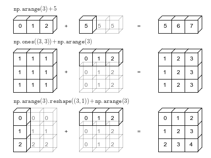
Matlab and Numpy automatically do this now.
Also (and previously) in matlab, e.g.: "brcm(@plus, A, x). numpy.broadcast
For true "Matrix-vector" multiplication, use matmul or "@"
a special case of matrix-matrix multiplication
w = np.array([[ 2, -6],
              [-1,  4]])
v = np.array([[+1],
              [-1]])
np.matmul(w,v)
w@v
Matrix-matrix multiplication
A = np.array([[1,2],[3, 4]])
B = np.array([[1,0],[1, 1]])
A*B
What is this doing?
np.matmul(A,B)
np.dot(A,B)
A@B
Reshaping vectors into matrices and whatever else you want
x = np.array([1,2,3,4])
x = x.reshape(4,1)
print(x.reshape(4,1))
print(x.reshape(2,2))
print(x)
x_T = x.transpose()
print (x_T)
print (x_T.shape)
print(x.T)
Famous matrices in NumPy
np.eye(3)
D = np.diag([1,2,3])
print(D)
np.diag(D)
NumPy Inverse
A = np.array([[1,2],[4,5]])
iA = np.linalg.inv(A)
print(iA)
print(np.matmul(A,iA))
2.*8.
A = np.random.randint(0, 10, size=(3, 3))
A_inv = np.linalg.inv(A)
print(A)
print(A_inv)
print(np.matmul(A,A_inv))
Note that "hard zeros" rarely exist in real world due to limited numerical precision.
Eigenvalue Decomposition in NumPy
A = np.asarray([[.3,.1,.6],[.1,.3,.6],[.15,.15,.70]])

np.linalg.eig(A)
Note there's only one return
(u,s) = np.linalg.eig(A)
print(u)
print(s)
help(np.linalg.eig)
SVD in NumPy
np.linalg.svd(A)
Note outputs are U, S, and V-transposed
help(np.linalg.svd)
QR in NumPy
Q,R = np.linalg.qr(A)
print(Q)
#print(R)
np.dot(Q[:,2],Q[:,2])
Q.T@Q
help(np.linalg.qr)
Lab: Least-squares regression various ways
Load Boston house prices dataset.
Formulate linear system and try using inverse and pseudoinverse to solve.
from sklearn.datasets import load_boston
boston = load_boston()
print(dir(boston))
print(boston.data.shape)
print(boston.feature_names)
print(boston.DESCR)
Nonlinear regression
(easy way) - Linear regression after nonlinear transformation
Old: \begin{align} \mathbf y = \beta_0 + \beta_1 \mathbf x_{(1)} + \beta_2 \mathbf x_{(2)} +...+ \beta_n \mathbf x_{(n)} + \varepsilon , \; \; \; \mathbf x_{(i)} = \begin{bmatrix} x_{(i),1} \\x_{(i),2} \\ \vdots \\ x_{(i),m} \end{bmatrix} \end{align}
New: \begin{align} \mathbf y = \beta_0 + \beta_1 \mathbf x'_{(1)} + \beta_2 \mathbf x'_{(2)} +...+ \beta_n \mathbf x'_{(n)} + \varepsilon, \;\;\; \mathbf x'_{(i)} = \begin{bmatrix} f_{(i)}(x_1) \\f_{(i)}(x_2) \\ \vdots \\ f_{(i)}(x_m) \end{bmatrix} \end{align}
...Feature Engineering
Polynomial regression - simple powers of data
New model: $\mathbf y = \beta_0 + \beta_1 \mathbf x'_{(1)} + \beta_2 \mathbf x'_{(2)} +...+ \beta_n \mathbf x'_{(n)} + \varepsilon$
$$\mathbf x'_{(i)} = \begin{bmatrix} f_{(i)}(x_1) \\f_{(i)}(x_2) \\ \vdots \\ f_{(i)}(x_m) \end{bmatrix} = \begin{bmatrix} x_{1}^i \\x_{2}^i \\ \vdots \\ x_{m}^i \end{bmatrix}$$Exercise: write the model equations out for 3D case, i.e. $\bf x$ is just $x_1$, $x_2$, and $x_3$.
Polynomial regression
show_polyfit_ho_example_results(dosage,conc_noisy,(1,2,3,4,5,6));
