Mathematical Methods for Data Science

Keith Dillon
Spring 2020

Topic 3: Highlights of Linear Algebra

This topic:

1. Overview
2. Matrix Algebra & Vector spaces
3. LU decomposition
4. Orthogonal matrices
5. Eigenvectors and eigenvalues

Reading:

• CTM Chapter 11 (the SVD) (optional)
• Strang part I (Highlights of Linear Algebra)
• https://math.mit.edu/~gs/learningfromdata/
• https://ocw.mit.edu/courses/mathematics/18-065-matrix-methods-in-data-analysis-signal-processing-and-machine-learning-spring-2018/index.htm
• https://www.ms.u-tokyo.ac.jp/news/docs/mmmf_10.pdf

I. Overview

Five Basic Problems

• $Ax=b$ --> Find $x$
• $Ax = \lambda x$ --> Find $\lambda$ and $x$
• $Av = \sigma u$ --> Find $u$, $v$, and $\sigma$
• minimize $\frac{\Vert Ax \Vert^2}{\Vert x \Vert^2}$ --> Find $x$
• Factor the matrix $A$ --> find rows and columns of factors

Goal: understanding problem, not just solving it

When does a solution $x$ exist for $Ax=b$?

If $A$ is a matrix of data, what parts of that data are most important?

"Data Science meets Linear Algebra in the SVD" -Gilbert Strang

Key info: column spaces, null spaces, eigenvectors and singular vectors

Applications

• Least squares
• Fourier transforms
• Web search
• Regression
• Training deep neural networks

II. Matrix Algebra & Vector Spaces

Vector space I

A vector space is a set of vectors with three additional properties (that not all sets of vectors have).

1. Contains origin
2. Closed under addition (of members of set)
3. Closed under scalar multiplication (of a member in the set)

Vector space II

Start with a set of vectors

$$ S = \{\mathbf v_1, \mathbf v_2, ..., \mathbf v_n\} $$

A vector space is a new set consisting of all possible linear combinations of vectors in $S$.

This is called the span of a set of vectors:

\begin{align} V &= Span(S) \\ &= \{\alpha_1 \mathbf v_1 + \alpha_2 \mathbf v_2 + ... + \alpha_n \mathbf v_n \text{ for all } \alpha_1,\alpha_2,...,\alpha_n \in \mathbf R\} \end{align}

If the vectors in $S$ are linearly independent, they form a basis for $V$.

The dimension of a vector space is the cardinality of (all) its bases.

Example: Column space (of a matrix $\mathbf A$)

Treat matrix as set of vectors defined by columns, and define vector space spanned by this set:

$$ \mathbf A \rightarrow S = \{ \mathbf a_1, \mathbf a_2, ..., \mathbf a_n \} $$$$ \text{Columnspace a.k.a. } C(\mathbf A) = Span(S) $$

Using definition of Span we can write: \begin{align} Span(S) &= \{\alpha_1 \mathbf a_1 + \alpha_2 \mathbf a_2 + ... + \alpha_n \mathbf a_n \text{ for all } \alpha_1,\alpha_2,...,\alpha_n \in \mathbf R\} \\ &= \{ \mathbf A \boldsymbol\alpha \text{ for all } \boldsymbol\alpha \in \mathbf R^n\} \end{align}

Where we defined $\boldsymbol\alpha$ as vector with elements $\alpha_i$.

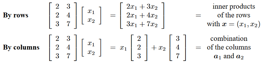
Multiplication $Ax$ using columns of $A$

Consider a 3x2 matrix $A$ multiplied by a 2x1 vector $x$

1. Via dot products of rows of $A$ with $x$
2. As linear combination of columns of $A$

Column space of $A$

The set of all possible linear columns $Ax$.

Draw this space for 3x2 $A$.

Solution of $Ax=b$

Column space: the set of $Ax$ for all possible $x$

Solution: the $x$ for which $Ax=b$.

...so when does $x$ exist? (and when does $x$ not exist?)

A solution $x$ exists iff $b$ is in the column space of $A$. (draw it).

Subspaces of $\mathbb R^3$

Consider column spaces formed by all possible linear combination of $n$ (linearly independent) columns. What shape are they?

• $n=0$

• $n=1$

• $n=2$

• $n=3$

Linear independence

A set of vectors is linearly dependent if one can be written as a linear combination of the others.

What happens for the previous subspace cases?

Basis (of the column space of $A$)

A linearly independent set of vectors which span the same space as the columns of $A$

Algorithm for finding basis given set of columns by construction:

• start with an empty set $C$
• select a column $a$ from $A$
• test if $a$ is linearly depndent on columns in $C$
• if it is, add $a$ to set $B$, otherwise discard $a$
• repeat with each of the remaining columns of $A$

Dimension & Rank

The dimension of a space is the cardinality of a (every) basis

The rank of a matrix the dimension of its column spac

Row-reduced Echelon Form

Consider the basis $C$ for the column space of $A$

Every column in $A$ can be written as a linear combination of the columns in $C$

Express these relationships as matrices, with the linear combination coefficients as columns in a matrix $R$

$R$ = rref($A$) = reduced row echelon form

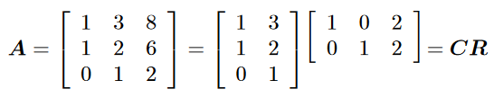
Our first factorization of $A$

Recall: Row echelon form

$$ \begin{pmatrix} 1 & a & b & c \\ 0 & 0 & 1 & d \end{pmatrix} $$

• Perform Gaussian elimination on rows to put pivots (first nonzero number in row) in increasing order
• "Reduced": pivot = 1
• This is a matrix description of our little construction algorithm!

• Why is there a 1 in the upper left (from our algorithm)?
• Why are there two leading zeros in the second row in this case?

Row rank vs. Column rank

• row rank is the number of independent rows, which is the number of rows in $R$
• column rank is the number of independent columns, which is the number of columns in $C$

where $A=CR$. How do these numbers relate?

Matrix-Matrix multiplication $AB = C$

Three "methods" now

1. Elements of $C$ as dot products of rows and columns
2. Columns of $C$ as linear combinations of rows of $A$
3. $C$ as sum of outer products

1. Elements of $C$ as dot products of rows and columns

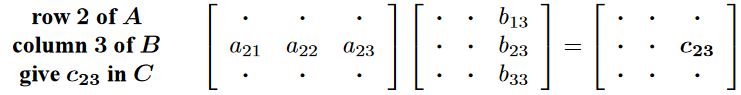
What is the equation for this? I.e. $C_{i,j} = ?$

2. Columns of $C$ as linear combinations of rows of $A$

Derive equation for this from previous version

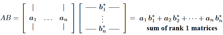
3. $C$ as sum of outer products

Recall: Outer product of vectors

$$ w = uv^T$$

All columns are multiples of $u$.

All rows are multiples of $v^T$

...Therefore $C$ as sum of outer products

Derive directly from matrix multiplication equation

$2 \times 2$ example on page 10

Value of outer-product perspective

Consider rank-1 matrices as components, some tiny some large

For data science we usually want the most important info in the data, i.e. most important components

Common theme: factoring matrix $A = CR$ and look components $c_kr_k^T$

Four Fundamental Subspaces

The "big picture" of linear algebra

• Column space $C(A)$ = all linear combos of the columns of $A$
• Rowspace $C(A^T)$ = all linear combos of the rows of $A$, i.e. columns of $A^T$
• Nullspace $N(A)$ = all vectors $Ax$
• Left nullspace $N(A^T)$ = all vectors $A^Tx$

Example 1 pg. 14, rank-1 matrix

$$A = \begin{pmatrix}1 &2\\3 &6\end{pmatrix} = uv^T$$

What are:

• column space
• row space
• null space
• left nullspace

Example 2 pg. 15, rank-1 matrix

$$B = \begin{pmatrix}1 &-2 &-2\\3 &-6 &-6\end{pmatrix} = uv^T$$

What are:

• column space
• row space
• null space
• left nullspace

Counting Law

$r$ independent equations $Ax=0$ (where $A$ is $m \times n$) have $n-r$ independent solutions

(Rank-nullity theorem)

• Dim of rowspace = dim of column space = $r$

• Dim of nullspace = $n-r$

• Dim of left nullspace = $m-r$

Note asymmetry of the left vs. right nullspaces

Example 3, pg. 16, Graph Incidence Matrix

Row of incidence matrix describes an edge

• $A_{ij} = -1$ means edge $i$ starts at node $j$
• $A_{ij} = +1$ means edge $i$ ends at node $j$
• hence rows sum to zero, so nullspace contains $(1,1,1,1)^T$ -- test by computing $Ax=0$

A linearly dependent set of rows (i.e. a solution to $A^Ty = 0$) forms a loop

Graph Incidence matrix subspaces

• $N(A) =\mathbf 1$, 1D nullspace is constant
• $C(A^T)$ = edges of tree, rank $=r=n-1$, independent rows
• $C(A)$ solutions to $Ax=0$, "voltage law"
• $N(A^T)$, solutions to $A^Tx=0$, loop currents... "current law"

Ranks: key facts

1. $rank(AB) \le rank(A)$, $rank(AB) \le rank(B)$
2. $rank(A+B) \le rank(A)+rank(B)$
3. $rank(A^TA) = rank(AA^T) = rank(A) =rank(A^T)$
4. if $m\times r$ $A$ is rank $r$ and $r\times m$ $B$ is rank $r$, then $AB$ is rank $r$

Recall can compute rank as number of independent columns, so consider columns of sum or product for above facts

III. LU Decomposition

Five important factorizations

• $A = LU$
• $A = QR$
• $S = Q\Lambda Q^T$
• $A = X\Lambda X^{-1}$
• $A = U\Sigma V^T$

Elimination and $LU$

Most fundamental problem of linear algebra: solve $Ax=b$

Assume square $A$ is $n \times n$ and and $x$ is $n \times 1$, so $n$ equations and $n$ unknowns.

1. use first equation to create zeros below first pivot
2. use next equation to create zeros below next pivot
3. continue until have produced an upper triangular matrix $U$

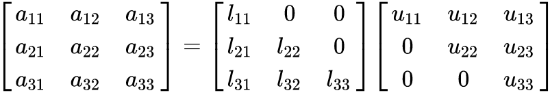
Triangular matrix

• Upper triangular $\mathbf U$ (a.k.a. $\mathbf R$)

  

• Lower triangular $\mathbf L$. What is $\mathbf L^T$?

  

Next step...

Elimination: $[A | b] = [LU | b] \rightarrow [U|L^{-1}b] = [U|c] $

Back substitution: solve $Ux = c$ (easy since $U$ is triagonal) to get $x = U^{-1}c = U^{-1}L^{-1}b = A^{-1}b$

Triangular matrix - Value

• can easily solve linear system $\bf Ux=c$

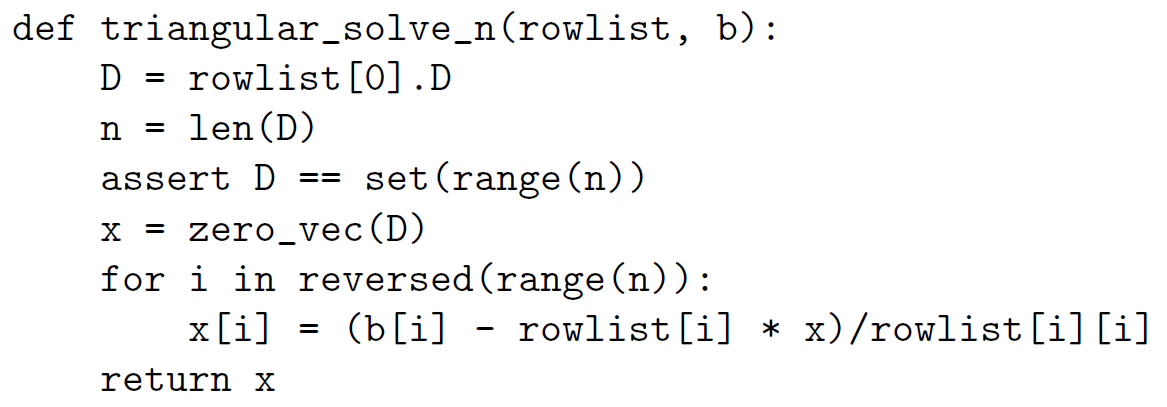
• note problem if have zero on diagonal

The $L$ matrix

• $L$ contains the multipliers we apply to the pivot to form $U$.
• View as parameters in a program we create from top row working downward
• $L_{ii} = 1$. we directly use the pivot value without scaling it
• $L_{ki}$ for $k>i$ is the number we scaled the pivot in row $i$ by to zero out element $ki$ in a lower row

Row Exchanges, a.k.a. Permutations

• Above algorithm assumes we had nonzero pivots, otherwise we'd need to reordre rows to get one
• General approach: choose largest number in column for pivot and reorder
• Permutation matrix - identiy matrix with rows (or equivalently columns) reordered
• General decomposition algorithm $PA = LU$

Applications of LU

• Solving linear systems (Elimination followed by subsitution)
• Computing determinant - $\det A = \det(PLU) = \det P \det L \det U = (-1)^p\prod_i L_{ii}U_{ii}$
• Inverting matrices

Basically all take advantage of ease of dealing with triangular matrices

IV. Orthogonal Vectors & Matrices

Orthogonal vectors

• Extension of idea of perpendicular vectors
• Orthogonal vectors $x$ and $y$.
• Test is $x^Ty = 0$

Law of Cosines

$$\Vert x-y\Vert^2 = \Vert x\Vert^2 + \Vert y\Vert^2 - \Vert x\Vert\Vert y\Vert\cos\theta$$

Orthogonal basis for a subspace,

• $\{v_i, v_2, ..., v_k\}$ where $v_i^Tv_j = 0$ for $i\ne j$
• $v_i^Tv_i = \Vert v_i \Vert^2$.
• if unit vectors: $\Vert v_i \Vert^2 = 1$ $\rightarrow$ orthonormal basis

Standard Basis for $\mathbb R^3$

$$ i=\begin{pmatrix} 1\\ 0\\ 0 \end{pmatrix}, \; j=\begin{pmatrix} 0\\ 1\\ 0 \end{pmatrix}, \; k=\begin{pmatrix} 0\\ 0\\ 1 \end{pmatrix}$$

Orthogonal subspaces

$R$ and $N$ where for every $u\in R$ and $v \in N$ $u^Tv=0$

Example: rowspace and nullspace of a matrix

Nullspace: $Ax=0$ directly implies $row\cdot x = 0$

Tall thin matrix $Q$ with orthonormal columns

$$Q^TQ = I$$$$\left(Q^TQ\right)_{ij} = q_i^Tq_j = \begin{cases} 1, i=j \\ 0, i\ne j \end{cases} $$

where $q_i$ is the $i^{th}$ column of $Q$

$$\Vert Qx\Vert = \sqrt{(Qx)^T(Qx)} = \sqrt{x^TQ^TQx} = \sqrt{x^TQ^TQx} = \sqrt{x^TIx} = \sqrt{x^Tx} = \Vert x \Vert$$

So $Q$ doesn't change the length of a vector

Projection matrix

$$P = QQ^T$$

$Pb$ is the orthogonal projection of $b$ onto the column space of $P$

Recall from physics, orthogonal unit vectors $\hat{x}$, $\hat{y}$, $\hat{z}$, use as columns of $P$

Key property of projection matrix: $P^2 = P$

Exercise: prove this

"Orthogonal matrices"

• square matrix with othonormal columns $Q^TQ = I$ so $Q^{-1} = Q^T$
• left inverse and right inverse
• columns are an orthonormal basis for $\mathbb R^n$
• rows also are an orthonormal basis for $\mathbb R^n$ (can be same one or different)
• should be called "orthonormal matrix"

Example: Rotation matrix

$$Q_{\theta} = \begin{pmatrix} \cos\theta & -\sin\theta \\ \sin\theta & \cos\theta \end{pmatrix}$$

Rotates a vector by $\theta$

Example: Reflection matrix

$$Q_{\theta} = \begin{pmatrix} \cos\theta & \sin\theta \\ \sin\theta & -\cos\theta \end{pmatrix}$$

Reflects a vector about line at angle $\frac{1}{2}\theta$

Coordinates

An orthogonal basis $\{q_1, ..., q_n\}$ can be viewed as axes of a coordinate system in $\mathbb R^n$

The coordinates within this system of a vector $v$ are the coefficients $c_i = q_i^T v$

Suppose $q_i$ are the rows of a matrix $Q$ (which is therefore an orthogonal matrix)

How do we compute $c_i$ given $v$ and $Q$?

Example: Householder Reflections

Reflection matrices $Q = H_n$

Defined as Identity matrix minus projection onto a given unit vector $u$... basically flip this component

Ex: $u = \frac{1}{\sqrt{n}}ones(n,1)$, $H_n = I - 2uu^T = I - ones(n,n)$

V. Eigenvalues and Eigenvectors

Eigenvector equation

$$Ax = \lambda x$$

• $x$ is eigenvector of $A$
• $\lambda$ is eigenvalue of $A$
• Eigenvectors don't change direction when multiplied by $A$, they only get scaled

Exercise: find eigenvectors and eigenvalues for $A^k$ in terms of those from $A$

Exercise: find eigenvectors and eigenvalues for $A^{-1}$ in terms of those from $A$

Properties

• $trace(A) = $ sum of eigenvalues
• $det(A) = $ product of eigenvalues
• Symmetric matrices have real eigenvalues
• If two eigenvalues differ, the corresponding eigenvectors are orthogonal
• Eigenvectors of a real matrix $A$ are orthogonal iff $A^TA = AA^T$

Example: Eigenvalues of Rotation

$$Q = \begin{pmatrix}0 &-1\\1 & 0\end{pmatrix}$$

Eigenvalues are $i$ and $-i$ for eigenvectors $\begin{pmatrix}1\\-i\end{pmatrix}$ and $\begin{pmatrix}1\\i\end{pmatrix}$. Test this.

Note that for complex vectors we define the inner product as $u^Hv$, conjugate transpose.

Eigenvalues of "shift"

Consider $A_s = A+sI$

What are the eigenvalues and eigenvectors of $A_s$ if we know $Ax=\lambda x$?

Similar Matrices

Consider $A_B = BAB^{-1}$, where $B$ is an invertible matrix

$A_B$ and $A$ are called similar matrices

How do the eigenvalues of similar matrices relate?

Diagonal matrix

$$D = \begin{bmatrix} D_{1,1} & 0 & 0\\ 0 & D_{2,2} & 0 \\ 0 & 0 & D_{3,3}\\ \end{bmatrix}$$

Can completely describe with a vector $\mathbf d$ with $d_i = D_{i,i}$

Hence we write "$\mathbf D = \text{diag}(\mathbf d)$" and "$\mathbf d = \text{diag}(\mathbf D)$"

Relate to Hadamard product of vectors $\mathbf D \mathbf v = \mathbf d \odot \mathbf v$.

Diagonalizing a matrix

Suppose we have $n$ independent eigenvectors for $Ax_i=\lambda_i x_i$, $i=1,...,n$

Combine these into the matrix decomposition $A = X\Lambda X^{-1}$

What are the properties of $X$ and $\Lambda$?

Construction of a matrix with specified Eigenvectors

Another illustration of diagonalization is the fact that the diagonalization formula can also be used to construct a matrix that has specified eigenvalues and eigenvectors.

Example:

Let $\lambda_1 = -1$ and $\lambda_2 = 2$ be the eigenvalues corresponding to the eigenvectors ${\bf u}_1 = \begin{bmatrix}5\\3\end{bmatrix}$ and ${\bf u}_2 = \begin{bmatrix}3\\2\end{bmatrix}$.

Find a matrix $\bf A$ which gives these eigenvalues and eigenvectors.

We start by constructing $\bf U$ and $\boldsymbol\Lambda$:

$${\bf U} = \left[ \begin{matrix} {\bf u}_1 & {\bf u}_2 \end{matrix} \right] = \left[ \begin{matrix} 5 & 3 \\ 3 & 2 \end{matrix} \right]~~~~\text{and}~~~~{\boldsymbol\Lambda} = \left[ \begin{matrix} \lambda_1 & 0 \\ 0 & \lambda_2 \end{matrix} \right] = \left[ \begin{matrix} -1 & 0 \\ 0 & 2 \end{matrix} \right]$$

Thus $${\bf U}^{-1} = \left[ \begin{matrix} 2 & -3 \\ -3 & 5 \end{matrix} \right]$$ This gives $${\bf A} = {\bf U}\boldsymbol\Lambda{\bf U}^{-1} = \left[ \begin{matrix} 5 & 3 \\ 3 & 2 \end{matrix} \right]\left[ \begin{matrix} \lambda_1 & 0 \\ 0 & \lambda_2 \end{matrix} \right]\left[ \begin{matrix} 2 & -3 \\ -3 & 5 \end{matrix} \right] = \left[ \begin{matrix} -28 & 45 \\ -18 & 29 \end{matrix} \right]$$

Check that these satisfy the eigenvector equation.

Check:

$${\bf A u}_1 = \left[ \begin{matrix} -28 & 45 \\ -18 & 29 \end{matrix} \right] \left[ \begin{matrix} 5 \\ 3 \end{matrix} \right] = \left[ \begin{matrix} -5 \\ -3 \end{matrix} \right] = (-1)\left[ \begin{matrix} 5 \\ 3 \end{matrix} \right]$$$${\bf A u}_2 = \left[ \begin{matrix} -28 & 45 \\ -18 & 29 \end{matrix} \right] \left[ \begin{matrix} 3 \\ 2 \end{matrix} \right] = \left[ \begin{matrix} 6 \\ 4 \end{matrix} \right] = (2)\left[ \begin{matrix} 3 \\ 2 \end{matrix} \right]$$

Hence $\lambda_1$ and $\lambda_2$ are eigenvalues of $\bf A$ associated with eigenvectors ${\bf u}_1$ and ${\bf u}_2$

Example: Defective matrix

Suppose we DON'T have $n$ independent eigenvectors for $Ax_i=\lambda_i x_i$, $i=1,...,n$

$$A = \begin{pmatrix}3 &1\\0 & 3\end{pmatrix}$$

Compute the eigenvalues and eigenvectors

Symmetric Matrices

Properties

• All $n$ eigenvalues of a symmetric matrix $S$ are real numbers
• The $n$ eigenvectors can be chosen orthogonal - and orthonormal

Example: Identity Matrix $I$

• Eigenvalues are all 1
• Any nonzero vector $x$ is an eigenvector: $Ix = 1x$

Therefore we choose to pick orthonormal eigenvectors

Spectral Theorem

For every real symmetric matrix $S$ we can decompose as

$$S = Q \Lambda Q^T$$

Where $Q$ is orthonormal and $\Lambda$ is diagonal and real.

Exercise: test symmetry of $Q \Lambda Q^T$

Applications of eigendecomposition $S = Q \Lambda Q^T$

Use it to:

• solve $Ax=b$
• Find inverse of matrix $A$

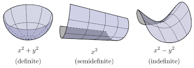
Positive Definiteness

• all positive eigenvalues = Positive definite matrix
• all non-negative eigenvalues = Positive semi-definite matrix

"Energy-based definition" - Positive definite matrix $S$ has $x^TSx>0$ for all $x\ne 0$

Examples (compute $x^TSx$)

$$S = \begin{pmatrix}2 &0\\0 & 6\end{pmatrix}$$

$$S = Q\begin{pmatrix}2 &0\\0 & 6\end{pmatrix}Q^T$$

Proving $x^TSx>0$ for all $x\ne 0$

$$Sx = \lambda x$$

multiply both sides by $s^T$

Exercise: prove $S_1+S_2$ is PD if both $S_1$ and $S_2$ are PD

"$AA^T$ test"

A symmetric Positive definite matrix $S$ can be factored as

$$S=AA^T$$

Where $A$ has independent columns.

There are many possible choices for $A$

Consider $A=Q\sqrt{\Lambda}Q^T = A^T$ (a matrix "square root")

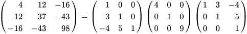
Cholesky Factorization

$A = LDL^T$, where $D$ is diagonal and $L$ comes from $LU$ decomposition.

Algorithms take advantage of symmetry so roughly twice as fast as $LU$.

Same handy uses as $LU$ otherwise.

Optimization

Surface described by $x^TSx$ is elliptical and has a unique minimum when $S$ is PD

Axes described by eigenvectors and eigenvalues. Consider diagonalization as coordinate transform.

Recap - general real square matrix $A$

• eigenvalues may be complex
• eigenvectors may not be independent (matrix is called "defective")
• if not defective, can form decomposition $A = X\Lambda X^{-1}$ (a.k.a. diagonalize)
• if eigenvalues are nonzero (i.e. matrix is also non-singular), can form inverse, $LU$ decomposition

Recap - Symmetric real matrix

• real eigenvalues
• can always diagonalize $A = X\Lambda X^{-1} = Q\Lambda Q^T$ (i.e. X is orthonormal matrix $Q$)

Recap - Symmetric real Positive definite matrix

• Has real positive eigenvalues
• Can generally form decomposition $A = BB^T$
• Can find Cholesky decomposition $A=LU$ or "LDL" decomposition $A=LDL^T$
• the quadratic form $x^TAx$ is always positive if $x \ne 0$, and has a unique minimum when $x=0$

SVD Motivation: Rectangular matrices

(particularly non-square real matrices)

$$A_{tall} = \begin{pmatrix}2 &0\\1 & 2\\5 &0\end{pmatrix}, \,\, A_{fat} = \begin{pmatrix}1 &3 &1\\2 & 0 & 1\end{pmatrix} $$

• $Ax=b$ is essentially same as a system with a square matrix that isn't full rank*
• $Ax = \lambda x$ isn't solvable

SVD: Singular vectors

• Replace $Ax = \lambda x$ with $Av = \sigma u$
• $n$ right singular vectors $v_1, ..., v_n$
• $m$ left singular vectors $u_1, ..., u_m$