Mathematical Methods for Data Science

Keith Dillon
Spring 2020

Topic 3: Norms, Distances, and Statistics

This topic:

1. Norms & Distances
2. Simple distance-based classification
3. Statistics
4. Preprocessing data

Reading:

• Coding the Matrix Chapter 8
• Strang I.11
• Strang Part V

Norms

A norm is a vector "length". Often denoted as $\Vert \mathbf x \Vert$.

Similar properties required.

1. Non-negativity: $\Vert \mathbf x \Vert \geq 0$
2. Zero upon equality: $\Vert \mathbf x \Vert = 0 \iff \mathbf x = \mathbf 0$
3. Absolute scalability: $\Vert \alpha \mathbf x \Vert = |\alpha| \Vert \mathbf x \Vert$ for scalar $\alpha$
4. Triangle Inequality: $\Vert \mathbf x + \mathbf z\Vert \leq \Vert \mathbf x\Vert + \Vert \mathbf z\Vert$

Famous norms

• $\ell_2$ norm
• $\ell_1$ norm
• $\ell_\infty$ norm
• $\ell_p$ norm
• "$\ell_0$" norm

Note we often lazily write these as e.g. "L2" norm, though mathematicians will complain because that mas a slightly different meaning already.

Norms and Lebesgue space

The $L^{p}$, or Lebesgue space, consists of all of functions of the form:

$\|f\|_{p} = (|x_{1}|^{p}+|x_{2}|^{p}+|x_{n}|^{p}+)^{1/p}$

This mathematical object is known as a p-norm.

$p$-norm: For any $n$-dimensional real or complex vector. i.e. $x \in \mathbb{R}^n \text{ or } \mathbb{C}^n$

$$ \|x\|_p = \left(|x_1|^p+|x_2|^p+\dotsb+|x_n|^p\right)^{\frac{1}{p}} $$$$ \|x\|_p = \begin{pmatrix}\sum_{i=1}^n{|x_i|^p} \end{pmatrix}^{\frac{1}{p}} $$

Consider the norms we have looked at. What is $p$?

Exercise

What are the norms of $\vec{a} = \begin{bmatrix}1\\3\\1\\-4\end{bmatrix}$ and $\vec{b} = \begin{bmatrix}2\\0\\1\\-2\end{bmatrix}$?

Distance Metrics

Ex: Euclidean distance between two vectors $a$ and $b$ in $\mathbb{R}^{n}$:

$$d(\mathbf a,\mathbf b) = \sqrt{\sum_{i=1}^{n}(b_i-a_i)^2}$$

But this may not make sense for flower dimensions. Many alternatives...

A metric $d(\mathbf x,\mathbf y)$ must satisfy four particular conditions to be considered a metric:

1. Non-negativity: $d(\mathbf x,\mathbf y) \geq 0$
2. Zero upon equality: $d(\mathbf x,\mathbf y) = 0 \iff \mathbf x = \mathbf y$
3. Commutativity of arguments: $d(\mathbf x,\mathbf y) = d(\mathbf y,\mathbf x)$
4. Triangle Inequality: $d(\mathbf x,\mathbf z) \leq d(\mathbf x,\mathbf y) + d(\mathbf y,\mathbf z)$

Norm versus Distance

What is the relationship?

Exercise

Write the Euclidean norm entirely in terms of dot products.

What does this tell you about using dot products to compare vector similarity?

Manhattan or "Taxicab" Distance, also "Rectilinear distance"

Measures the relationships between points at right angles, meaning that we sum the absolute value of the difference in vector coordinates.

This metric is sensitive to rotation.

$$d_{M}(a,b) = \sum_{i=1}^{n}|b_i-a_i|$$

Exercise

Does it fulfill the 4 conditions?

Manhattan or "Taxicab" Distance, also "Rectilinear distance"

Measures the relationships between points at right angles, meaning that we sum the absolute value of the difference in vector coordinates.

This metric is sensitive to rotation.

$$d_{M}(a,b) = \sum_{i=1}^{n}|(b_i-a_i)|$$

1. Non-negativity: $d(\mathbf x,\mathbf y) \geq 0$
2. Zero upon equality: $d(\mathbf x,\mathbf y) = 0 \iff \mathbf x = \mathbf y$
3. Commutativity of arguments: $d(\mathbf x,\mathbf y) = d(\mathbf y,\mathbf x)$
4. Triangle Inequality: $d(\mathbf x,\mathbf z) \leq d(\mathbf x,\mathbf y) + d(\mathbf y,\mathbf z)$

Chebyschev Distance

The Chebyschev distance or sometimes the $L^{\infty}$ metric, between two vectors is simply the the greatest of their differences along any coordinate dimension:

$$d_{\infty}(\mathbf a,\mathbf b) = \max_{i}{|(b_i-a_i)|}$$

Chebyschev Distance

The Chebyschev distance or sometimes the $L^{\infty}$ metric, between two vectors is simply the the greatest of their differences along any coordinate dimension:

$$d_{\infty}(\mathbf a,\mathbf b) = \max_{i}{|(b_i-a_i)|}$$

1. Non-negativity: $d(\mathbf x,\mathbf y) \geq 0$
2. Zero upon equality: $d(\mathbf x,\mathbf y) = 0 \iff \mathbf x = \mathbf y$
3. Commutativity of arguments: $d(\mathbf x,\mathbf y) = d(\mathbf y,\mathbf x)$
4. Triangle Inequality: $d(\mathbf x,\mathbf z) \leq d(\mathbf x,\mathbf y) + d(\mathbf y,\mathbf z)$

Cosine Distance

Only depends on angle between the vectors

$$d_{Cos}(\mathbf a,\mathbf b) = 1-\frac{\mathbf a \cdot \mathbf b}{\|\mathbf a\|\|\mathbf b\|}$$

Not a true distance metric. which propery fails to hold? (easy to guess at based on geometry)

Exercise

Implement the metrics manually and compute distances between:

$ \begin{bmatrix} 1 \\ 2 \\ 3 \\ 4 \end{bmatrix}$ and $ \begin{bmatrix} 5 \\ 6 \\ 7 \\ 8 \end{bmatrix}$

II. Distance-based Classification

Lab: simple classification with distances

Load and investigate the IRIS dataset from scikit.

Imagine we flower measurements for one of the flowers but don't know the flower type. We want to classify its type by finding the flower of known type which is most similar.

Do this by taking each flower and computing a distance metric between its measurements and that of every other flower. Take the type of the "nearest" flower as your estimate of the flower type.

Compute the accuracy of this technique based on how many flowers are classified correctly in this way.

Try using different distance metrics to compare flowers. Which makes most sense?

from sklearn import datasets
iris = datasets.load_iris()

dir(iris)

['DESCR', 'data', 'feature_names', 'filename', 'target', 'target_names']

(iris.data, iris.target)

(array([[5.1, 3.5, 1.4, 0.2],
        [4.9, 3. , 1.4, 0.2],
        [4.7, 3.2, 1.3, 0.2],
        [4.6, 3.1, 1.5, 0.2],
        [5. , 3.6, 1.4, 0.2],
        [5.4, 3.9, 1.7, 0.4],
        [4.6, 3.4, 1.4, 0.3],
        [5. , 3.4, 1.5, 0.2],
        [4.4, 2.9, 1.4, 0.2],
        [4.9, 3.1, 1.5, 0.1],
        [5.4, 3.7, 1.5, 0.2],
        [4.8, 3.4, 1.6, 0.2],
        [4.8, 3. , 1.4, 0.1],
        [4.3, 3. , 1.1, 0.1],
        [5.8, 4. , 1.2, 0.2],
        [5.7, 4.4, 1.5, 0.4],
        [5.4, 3.9, 1.3, 0.4],
        [5.1, 3.5, 1.4, 0.3],
        [5.7, 3.8, 1.7, 0.3],
        [5.1, 3.8, 1.5, 0.3],
        [5.4, 3.4, 1.7, 0.2],
        [5.1, 3.7, 1.5, 0.4],
        [4.6, 3.6, 1. , 0.2],
        [5.1, 3.3, 1.7, 0.5],
        [4.8, 3.4, 1.9, 0.2],
        [5. , 3. , 1.6, 0.2],
        [5. , 3.4, 1.6, 0.4],
        [5.2, 3.5, 1.5, 0.2],
        [5.2, 3.4, 1.4, 0.2],
        [4.7, 3.2, 1.6, 0.2],
        [4.8, 3.1, 1.6, 0.2],
        [5.4, 3.4, 1.5, 0.4],
        [5.2, 4.1, 1.5, 0.1],
        [5.5, 4.2, 1.4, 0.2],
        [4.9, 3.1, 1.5, 0.2],
        [5. , 3.2, 1.2, 0.2],
        [5.5, 3.5, 1.3, 0.2],
        [4.9, 3.6, 1.4, 0.1],
        [4.4, 3. , 1.3, 0.2],
        [5.1, 3.4, 1.5, 0.2],
        [5. , 3.5, 1.3, 0.3],
        [4.5, 2.3, 1.3, 0.3],
        [4.4, 3.2, 1.3, 0.2],
        [5. , 3.5, 1.6, 0.6],
        [5.1, 3.8, 1.9, 0.4],
        [4.8, 3. , 1.4, 0.3],
        [5.1, 3.8, 1.6, 0.2],
        [4.6, 3.2, 1.4, 0.2],
        [5.3, 3.7, 1.5, 0.2],
        [5. , 3.3, 1.4, 0.2],
        [7. , 3.2, 4.7, 1.4],
        [6.4, 3.2, 4.5, 1.5],
        [6.9, 3.1, 4.9, 1.5],
        [5.5, 2.3, 4. , 1.3],
        [6.5, 2.8, 4.6, 1.5],
        [5.7, 2.8, 4.5, 1.3],
        [6.3, 3.3, 4.7, 1.6],
        [4.9, 2.4, 3.3, 1. ],
        [6.6, 2.9, 4.6, 1.3],
        [5.2, 2.7, 3.9, 1.4],
        [5. , 2. , 3.5, 1. ],
        [5.9, 3. , 4.2, 1.5],
        [6. , 2.2, 4. , 1. ],
        [6.1, 2.9, 4.7, 1.4],
        [5.6, 2.9, 3.6, 1.3],
        [6.7, 3.1, 4.4, 1.4],
        [5.6, 3. , 4.5, 1.5],
        [5.8, 2.7, 4.1, 1. ],
        [6.2, 2.2, 4.5, 1.5],
        [5.6, 2.5, 3.9, 1.1],
        [5.9, 3.2, 4.8, 1.8],
        [6.1, 2.8, 4. , 1.3],
        [6.3, 2.5, 4.9, 1.5],
        [6.1, 2.8, 4.7, 1.2],
        [6.4, 2.9, 4.3, 1.3],
        [6.6, 3. , 4.4, 1.4],
        [6.8, 2.8, 4.8, 1.4],
        [6.7, 3. , 5. , 1.7],
        [6. , 2.9, 4.5, 1.5],
        [5.7, 2.6, 3.5, 1. ],
        [5.5, 2.4, 3.8, 1.1],
        [5.5, 2.4, 3.7, 1. ],
        [5.8, 2.7, 3.9, 1.2],
        [6. , 2.7, 5.1, 1.6],
        [5.4, 3. , 4.5, 1.5],
        [6. , 3.4, 4.5, 1.6],
        [6.7, 3.1, 4.7, 1.5],
        [6.3, 2.3, 4.4, 1.3],
        [5.6, 3. , 4.1, 1.3],
        [5.5, 2.5, 4. , 1.3],
        [5.5, 2.6, 4.4, 1.2],
        [6.1, 3. , 4.6, 1.4],
        [5.8, 2.6, 4. , 1.2],
        [5. , 2.3, 3.3, 1. ],
        [5.6, 2.7, 4.2, 1.3],
        [5.7, 3. , 4.2, 1.2],
        [5.7, 2.9, 4.2, 1.3],
        [6.2, 2.9, 4.3, 1.3],
        [5.1, 2.5, 3. , 1.1],
        [5.7, 2.8, 4.1, 1.3],
        [6.3, 3.3, 6. , 2.5],
        [5.8, 2.7, 5.1, 1.9],
        [7.1, 3. , 5.9, 2.1],
        [6.3, 2.9, 5.6, 1.8],
        [6.5, 3. , 5.8, 2.2],
        [7.6, 3. , 6.6, 2.1],
        [4.9, 2.5, 4.5, 1.7],
        [7.3, 2.9, 6.3, 1.8],
        [6.7, 2.5, 5.8, 1.8],
        [7.2, 3.6, 6.1, 2.5],
        [6.5, 3.2, 5.1, 2. ],
        [6.4, 2.7, 5.3, 1.9],
        [6.8, 3. , 5.5, 2.1],
        [5.7, 2.5, 5. , 2. ],
        [5.8, 2.8, 5.1, 2.4],
        [6.4, 3.2, 5.3, 2.3],
        [6.5, 3. , 5.5, 1.8],
        [7.7, 3.8, 6.7, 2.2],
        [7.7, 2.6, 6.9, 2.3],
        [6. , 2.2, 5. , 1.5],
        [6.9, 3.2, 5.7, 2.3],
        [5.6, 2.8, 4.9, 2. ],
        [7.7, 2.8, 6.7, 2. ],
        [6.3, 2.7, 4.9, 1.8],
        [6.7, 3.3, 5.7, 2.1],
        [7.2, 3.2, 6. , 1.8],
        [6.2, 2.8, 4.8, 1.8],
        [6.1, 3. , 4.9, 1.8],
        [6.4, 2.8, 5.6, 2.1],
        [7.2, 3. , 5.8, 1.6],
        [7.4, 2.8, 6.1, 1.9],
        [7.9, 3.8, 6.4, 2. ],
        [6.4, 2.8, 5.6, 2.2],
        [6.3, 2.8, 5.1, 1.5],
        [6.1, 2.6, 5.6, 1.4],
        [7.7, 3. , 6.1, 2.3],
        [6.3, 3.4, 5.6, 2.4],
        [6.4, 3.1, 5.5, 1.8],
        [6. , 3. , 4.8, 1.8],
        [6.9, 3.1, 5.4, 2.1],
        [6.7, 3.1, 5.6, 2.4],
        [6.9, 3.1, 5.1, 2.3],
        [5.8, 2.7, 5.1, 1.9],
        [6.8, 3.2, 5.9, 2.3],
        [6.7, 3.3, 5.7, 2.5],
        [6.7, 3. , 5.2, 2.3],
        [6.3, 2.5, 5. , 1.9],
        [6.5, 3. , 5.2, 2. ],
        [6.2, 3.4, 5.4, 2.3],
        [5.9, 3. , 5.1, 1.8]]),
 array([0, 0, 0, 0, 0, 0, 0, 0, 0, 0, 0, 0, 0, 0, 0, 0, 0, 0, 0, 0, 0, 0,
        0, 0, 0, 0, 0, 0, 0, 0, 0, 0, 0, 0, 0, 0, 0, 0, 0, 0, 0, 0, 0, 0,
        0, 0, 0, 0, 0, 0, 1, 1, 1, 1, 1, 1, 1, 1, 1, 1, 1, 1, 1, 1, 1, 1,
        1, 1, 1, 1, 1, 1, 1, 1, 1, 1, 1, 1, 1, 1, 1, 1, 1, 1, 1, 1, 1, 1,
        1, 1, 1, 1, 1, 1, 1, 1, 1, 1, 1, 1, 2, 2, 2, 2, 2, 2, 2, 2, 2, 2,
        2, 2, 2, 2, 2, 2, 2, 2, 2, 2, 2, 2, 2, 2, 2, 2, 2, 2, 2, 2, 2, 2,
        2, 2, 2, 2, 2, 2, 2, 2, 2, 2, 2, 2, 2, 2, 2, 2, 2, 2]))

iris.data[52]

array([6.9, 3.1, 4.9, 1.5])

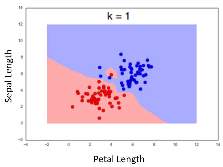
The "1-Nearest-Neighbor" Algorithm

Example using two features. Dots represent the measurements for the flowers in the dataset. Color of background is class of nearest neighbor (as if the point was the measurements for an unknown flower we were classifying)

Hamming or "Rook" Distance

The hamming distance can be used to compare nearly anything to anything else.

Defined as the number of differences in characters between two strings of equal length, ie:

$$d_{hamming}('bear', 'beat') = 1$$$$d_{hamming}('cat', 'cog') = 2$$$$d_{hamming}('01101010', '01011011') = 3$$

Edit distance

Similar to hamming distance, but also includes insertions and deletions, and so can compare strings of any length to each other.

$$d_{edit}('lead', 'gold') = 4$$$$d_{edit}('monkey', 'monk') = 2$$$$d_{edit}('lucas', 'mallori') = 8$$

• A kind of approximate matching method.
• Must use dynamic programming or memoization for efficiency

III. Statistics via Norms

Statistics

Consider the relation between norms and simple statistical quantities

\begin{align} \text{Population mean} &= \mu = \frac{\sum_{i=1}^N x_i}{N} \\ \text{Sample mean} &= \bar{x} = \frac{\sum_{i=1}^n x_i}{n} \\ \text{Population variance} &= \sigma^2 = \frac{\sum_{i=1}^N (x_i - \mu)^2}{N} \\ \text{Sample variance} &= s^2 = \frac{\sum_{i=1}^n (x_i - \bar{x})^2}{n - 1} = \frac{\sum_{i=1}^n x_i^2 - \frac{1}{n}(\sum_{i=1}^n x_i)^2}{n - 1} \\ \text{Standard deviation} &= \sqrt{\text{Variance}} \end{align}

More Statistics: Correlation(s)

\begin{align} \text{Variance } s^2 &= \frac{\sum_{i=1}^n (x_i - \bar{x})^2}{n - 1} = \frac{\sum_{i=1}^n x_i^2 - \frac{1}{n}(\sum_{i=1}^n x_i)^2}{n - 1} \\ \text{Standard deviation} &= \sqrt{\text{Variance}} \end{align}\begin{align} \text{Correlation Coefficient } r &= \frac{ \sum_{i=1}^n (x_i - \bar{x})(y_i - \bar{y})}{\sqrt{\sum_{i=1}^n(x_i - \bar{x})^2}\sqrt{\sum_{i=1}^n(y_i - \bar{y})^2}} = \frac{S_{xy}}{\sqrt{S_{xx} S_{yy}}} \\ %\text{''Corrected Correlation''} % &= S_{xy} = \sum_{i=1}^n (x_i - \bar{x})(y_i - \bar{y}) % = \sum_{i=1}^n x_i y_i - \frac{1}{n}(\sum_{i=1}^n x_i)(\sum_{i=1}^n y_i) \\ \text{Covariance} &= S_{xy} = \frac{1}{n-1}\sum_{i=1}^n (x_i - \bar{x})(y_i - \bar{y}) % = \sum_{i=1}^n x_i y_i - \frac{1}{n}(\sum_{i=1}^n x_i)(\sum_{i=1}^n y_i) \end{align}

Look kind of familiar? Relate to variance.

Exercise:

Assume you have a vector containing samples. Write the following in terms of norms and dot products:

1. mean
2. variance
3. Correlation coefficient
4. Covariance

So what does this tell you about comparing things using distances versus dot products versus statistics?

IV. Preprocessing Data

Preprocessing

We can now perform a variety of methods for preprocessing data.

Suppose we put our data (such as the Iris data) into vectors, one for each flower measurement ("feature").

We could:

• Remove the means (commonly done in many methods)
• Scale by 1/norm (often called "normalizing")

Standardizing a vector

1. remove the mean
2. Scale by 1/(standard deviation)

What is the mean and variance now?

"Standard" comes from standard normal distribution.

Lab: Normalizing data

Standardize the columns of the Iris dataset using linear algebra.

Test it worked by computing the mean and norm of each column.