Mathematical Methods for Data Science
Topic 4: The Singular Value Decomposition
This topic:
- Famous matrices review
- Famous spaces
- Rank-nullity and fundamental theorem of linear algebra
- Underdetermined and overdetermined linear systems
- Eigenvector decomposition
- The Singular value decomposition
Reading: CTM Chapter 10
Famous Matrices
- Triangular matrix
- Identity matrix
- Permutation matrix
- Diagonal matrix
- Orthogonal matrix
Famous Matrices: Triangular matrix
Upper triangular $\mathbf U$ (a.k.a. $\mathbf R$)

Lower triangular $\mathbf L$. What is $\mathbf L^T$?

Famous Matrices: Triangular matrix - Value
- can easily solve linear system $\bf Ax=b$
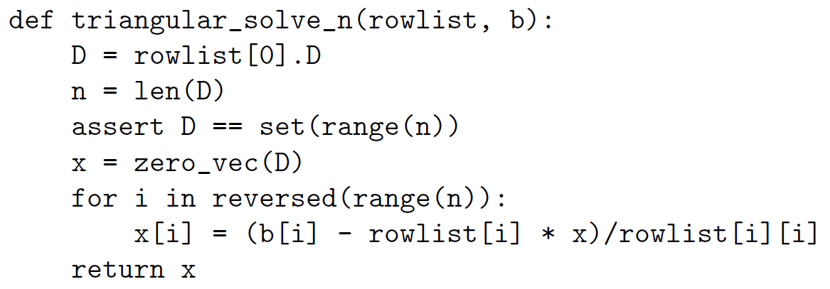
- note problem if have zero on diagonal
Exercise - implement the triangular solve algorithm
Famous Matrices: Identity matrix
$$I_3 = \begin{bmatrix} 1 & 0 & 0\\ 0 & 1 & 0 \\ 0 & 0 & 1\\ \end{bmatrix}$$Here we can write $\textit{I}\textit{B} = \textit{B}\textit{I} = \textit{B}$ or $\textit{I}\textit{I} = \textit{I}$.
Subscripts are sometimes used to denote size, since can have identities of all sizes.
Columns of $\mathbf I$ are handy vectors by themselves too, written as $\mathbf e_k$. What is $\mathbf e_k^T \mathbf v$ for some vector $\mathbf v$?
Famous Matrices: Permutation matrix
- Just identity with permuted columns.
Famous Matrices: Diagonal matrix
$$D = \begin{bmatrix} D_{1,1} & 0 & 0\\ 0 & D_{2,2} & 0 \\ 0 & 0 & D_{3,3}\\ \end{bmatrix}$$Can completely describe with a vector $\mathbf d$ with $d_i = D_{i,i}$
Hence we write "$\mathbf D = \text{diag}(\mathbf d)$" and "$\mathbf d = \text{diag}(\mathbf D)$"
Relate to Hadamard product of vectors $\mathbf D \mathbf v = \mathbf d \odot \mathbf v$.
import numpy as np

d = np.array([1,2,3,4])
D = np.diag(d)
print(D)
A = np.array([[1,2,3],[4,5,6],[7,8,9]])
print(A)
print(np.diag(A))
d = np.array([1,2,3,4])
D = np.diag(d)
x = np.array([3,3,3,3])
print(D@x)
print(d*x)
Famous Matrices: Diagonal matrix - Applications
Consider product $\mathbf D \mathbf v$
Consider products $\mathbf D \mathbf A$ and $\mathbf A \mathbf D$
Consider norm $\Vert \mathbf D \mathbf v \Vert_2$
Consider $\mathbf D_1 \mathbf D_2$
Consider power $\mathbf D^n$
Consider inverse of diagonal matrix $\bf D$
Solve linear system $\mathbf A \mathbf x = \mathbf b$ when $\mathbf A$ is diagonal.
d = np.array([1,2,3,4])
D = np.diag(d)
print(D)
print(np.linalg.inv(D))
d = np.array([1,2,0,4])
D = np.diag(d)
print(D)
print(np.linalg.inv(D))
print(np.linalg.pinv(D))
Famous Matrices: Orthogonal matrix
Square marix where columns are orthogonal, i.e. $\mathbf a_i^T \mathbf a_j = 0$ when $i \ne j$
Orthonormal matrix $\rightarrow$ also have $\mathbf a_i^T \mathbf a_i = 1$
Famous Matrices: Orthogonal matrix - Applications
Geometrically, orthonormal matrices implement rotations.
Very easy inverse
Solve linear system $\mathbf U \mathbf x = \mathbf b$ for $\mathbf x$ when $\mathbf U$ is orthonormal.
Solve matrix system $\mathbf U \mathbf A = \mathbf V$ for $\mathbf A$ when $\mathbf U$ is orthonormal.
Diagonalization
a.k.a. Eigendecomposition
a.k.a. Spectral Decomposition)
$$ {\bf A}{\bf U} = {\bf U} \boldsymbol\Lambda \rightarrow {\bf A} = {\bf U} \boldsymbol\Lambda {\bf U}^{-1} $$We can also solve for $\boldsymbol\Lambda$ = ?
Value of Diagonalizability
Assume $\bf A$ is diagonalizable, meaning we can find ${\bf A} = {\bf U}\boldsymbol\Lambda{\bf U}^{-1}$
Use this decomposition to solve ${\bf A}{\bf x}={\bf b}$
Value of Diagonalizability
Assume $\bf A$ is diagonalizable, meaning we can find ${\bf A} = {\bf U}\boldsymbol\Lambda{\bf U}^{-1}$
Use this decomposition to find the inverse of ${\bf A}$ (if you can)
Normal matrices: A new special matrix category
A real matrix $\bf A$ is a normal matrix if:
$$ \mathbf A \mathbf A^T = \mathbf A^T \mathbf A$$Note this must be a square and symmetric matrix due to matrix multiplication rules.
Examples of Normal matrices
Consider important special cases:
$\mathbf A = \mathbf B \mathbf B^T$ for some $m \times n$ matrix $\bf B$
$\mathbf A = \mathbf B^T \mathbf B$ for some $m \times n$ matrix $\bf B$
Test whether these work.
Value of Normal matrices
If a real matrix $\bf A$ is a normal matrix then its eigenvectors are orthonormal.
$$ {\bf A}{\bf U} = {\bf U} \boldsymbol\Lambda \rightarrow ? $$The Singular Value Decomposition (SVD)
Now we are back to talking about general rectangular matrices, not square, nor symmetric, nor normal, etc.
The SVD of a $m \times n$ matrix $\bf A$ is:
$${\bf A} = {\bf U S V}^T$$Where $\bf U$ and $\bf V$ are orthonormal matrices and $\bf S$ is a "rectangular diagonal matrix". E.g.
$${\bf S} = \left[ \begin{matrix} s_1 & 0 & \cdots & 0 \\ 0 & s_2 & \cdots & 0 \\ \vdots & \vdots & \ddots & \vdots \\ 0 & 0 & \cdots & s_m \\ \vdots & \vdots & \vdots & \vdots \\ 0 & 0 & \cdots & 0 \end{matrix} \right] \text{, or } {\bf S} = \left[ \begin{matrix} s_1 & 0 & \cdots & 0 & ... & 0 \\ 0 & s_2 & \cdots & 0 & ... & 0\\ \vdots & \vdots & \ddots & \vdots \\ 0 & 0 & \cdots & s_m & ... & 0\\ \end{matrix} \right] $$$s_i$ are the singular values of $\mathbf A$ and are sorted in decreasing order $s_1 \ge s_2 \ge ... \ge s_r$
The columns of $\bf U$ and $\bf V$ are the left and right singular vectors, respectively.
Exercise: SVD matrix sizes
Using matrix multiplication rules, work out the sizes of each component in the decomposition where $\bf A$ is $m \times n$
$${\bf A} = {\bf U S V}^T$$Draw a picture of what the shapes of the matrices look like.
Hint: orthonormal (and orthogonal) matrices are square.
Relation between SVD and Diagonalization
Now plug ${\bf A} = {\bf U S V}^T$, into the products $\mathbf M_1 = \mathbf A \mathbf A^T$ and $\mathbf M_2 = \mathbf A^T \mathbf A$.
What do you get?
Notice $\mathbf M_1$ and $\mathbf M_2$ are Normal matrices, so write their eigendecompositions.
...Tada! we have discovered a way to compute the SVD using eigenvalue decomposition methods.
NumPy Time
Form a random matrix with NumPY then compute its SVD and demonstrate you can reconstruct the original matrix by multiplying the component matrices together.
Note: Numpy.linalg.svd returns $\mathbf V^T$ (where other software like matlab returns $\mathbf V$
More Exercise
Form a random matrix with NumPY then compute eigendecompositions and SVD's to check the preceding relationships.
SVD and rank
The rank of a matrix is the number of nonzero singular values it has.
Test this by making a singular matrix in numpy then computing its svd and rank with nympy.
Famous Spaces
- $\mathbf R^n$
- Vector space
- column space
- row space
- null space
- left null space
Famous Spaces: Vector space I
A vector space is a set of vectors with three additional properties (that not all sets of vectors have).
- Contains origin
- Closed under addition (of members of set)
- Closed under scalar multiplication (of a member in the set)
Famous Spaces: Vector space II
Start with a set of vectors
$$ S = \{\mathbf v_1, \mathbf v_2, ..., \mathbf v_n\} $$A vector space is a new set consisting of all possible linear combinations of vectors in $S$.
This is called the span of a set of vectors:
\begin{align} V &= Span(S) \\ &= \{\alpha_1 \mathbf v_1 + \alpha_2 \mathbf v_2 + ... + \alpha_n \mathbf v_n \text{ for all } \alpha_1,\alpha_2,...,\alpha_n \in \mathbf R\} \end{align}If the vectors in $S$ are linearly independent, they form a basis for $V$.
The dimension of a vector space is the cardinality of (all) its bases.
Famous Spaces: Column space (of a matrix $\mathbf A$)
Treat matrix as set of vectors defined by columns, and define vector space spanned by this set:
$$ \mathbf A \rightarrow S = \{ \mathbf a_1, \mathbf a_2, ..., \mathbf a_n \} $$$$ \text{Columnspace a.k.a. } C(\mathbf A) = Span(S) $$Using definition of Span we can write: \begin{align} Span(S) &= \{\alpha_1 \mathbf a_1 + \alpha_2 \mathbf a_2 + ... + \alpha_n \mathbf a_n \text{ for all } \alpha_1,\alpha_2,...,\alpha_n \in \mathbf R\} \\ &= \{ \mathbf A \boldsymbol\alpha \text{ for all } \boldsymbol\alpha \in \mathbf R^n\} \end{align}
Where we defined $\boldsymbol\alpha$ as vector with elements $\alpha_i$.
Famous Spaces: Column space (of a matrix $\mathbf A$)
Now consider the set formed by rows of $\mathbf A$. What do you get for its span?
Famous Spaces: Null space (of a matrix $\mathbf A$)
Defined directly in matrix terms:
$$ Null(\mathbf A) = \{ \mathbf v : \mathbf A \mathbf v = \mathbf 0 \} $$Work the other direction and write this in terms of linear combinations. What is it saying about linear independence/dependence?
Famous Spaces: Left Null space (of a matrix $\mathbf A$)
Assuming a "symmetry" of ideas, what might this be?
Rank (of a matrix $\mathbf A$)
- row-rank = dimension of rowspace
- column-rank = dimension of column space
- Surprise! They're the same.
- Full rank = highest possible rank
- Consider a "full rank" square matrix. What is its nullity?
- Consider a "full rank" $m \times n$ (rectangular) matrix. What is its rank?
The Rank-Nullity theorem (of a $m \times n$ matrix $\mathbf A$)
Nullity defined as dimension of nullspace.
$$ Rank(\mathbf A) + Nullity(\mathbf A) = n $$Note that while rank is a "symmetric" concept, nullspace is specific to left or right.
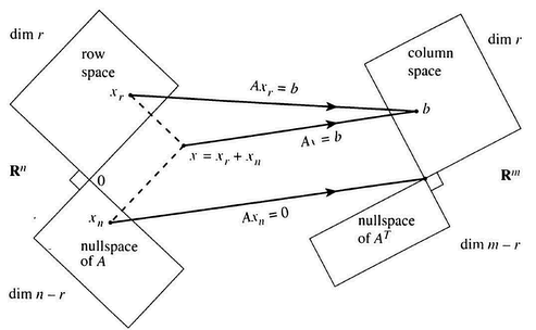
Four Fundamental Subspaces
Rank
- Treat the columns as a set (also works for rows)
- Find a basis for the span of the columns
- The size of this (and every other basis) is the rank of the matrix
What does it mean if the rank is smaller than the number of columns?
Rank-1 matrix
Suppose we have $n$ vectors $\{ \mathbf a_i \}$ but they all are in a subspace spanned by a single basis vector $\mathbf u$.
I.e. $\mathbf a_i = v_i \mathbf u$.
Form the matrix $\mathbf A$ who's columns are $\mathbf a_i$, in terms of vectors $\mathbf u$ and $\mathbf v$.
General Rank-1 matrix
$$ \mathbf A = \mathbf u \mathbf v^T $$Rank-2 matrix
Suppose we have $n$ vectors $\{ \mathbf a_i \}$ but they all are in a subspace spanned by two basis vectors $\mathbf u_1$ and $\mathbf u_2$.
I.e. $\mathbf a_i = v^{(1)}_i \mathbf u_1 + v^{(2)}_i \mathbf u_2$.
Form the matrix $\mathbf A$ who's columns are $\mathbf a_i$, in terms of vectors $\mathbf u_i$ and $\mathbf v_i$.
General Rank-2 matrix
$$ \mathbf A = \mathbf u_1 \mathbf v_1^T + \mathbf u_2 \mathbf v_2^T = "\mathbf U \mathbf V^T" $$Matrix multiplication method #3
$$\mathbf U \mathbf V^T = \sum_{i=1}^n \mathbf u_i \mathbf v_i^T$$where $\mathbf u_i$ are columns of $\mathbf U$ and $\mathbf v_i$ are columns of $\mathbf V$
Exercise
Make a pair of 2x2 matrices and test this works
SVD as Expansion
Apply this to the SVD ${\bf A} = {\bf U S V}^T$ and what do you get? (hint combine diaginal matrix with one of the others first).
Write down what each column of $\bf A$ looks like with this sum
SVD as expansion
So the SVD can be viewed as an expansion into rank-1 matrices
Each term inroduces components from an orthogonal basis vector
Each term gets progressively smaller (recall we have $s_1 \ge s_2 \ge ...$)
We can truncate this expansion to form an approximate version of matrix at chosen rank.
Four Fundamental Subspaces Again
Reconsider the column-space and Nullspace now using our expansion.
Take home messages:
The rank of $\mathbf A = \mathbf U \mathbf S \mathbf V^T$ is the number of nonzero singular values.
The column-space is spanned by the right singular vectors (columns of $\bf V$) corresponding to nonzero singular values.
The nullspace is spanned by the rest of the columns of $\bf V$.
The row-space is spanned by the left singular vectors (columns of $\bf U$) corresponding to nonzero singular values.
The left nullspace is spanned by the rest of the columns of $\bf U$.
Draw a picture describing this.
import numpy as np
A = np.array([[1,0,1],[0,1,1]])
np.linalg.svd(A)
A = np.array([[1],[2],[3]])@np.array([[1,1,0,1]])
A
np.linalg.svd(A)
np.linalg.matrix_rank(A)
np.array([[1],[2],[3]]).shape
np.array([[1,1,0,1]]).shape
np.array([1,1,0,1]).shape
Reduced form of the SVD
We can discard the columns of $U$ and $V$ and corresponding all-zero rows and cols of $S$ and get the same product
Eigenvalue Decomposition in NumPy
Exercises
Make a little matrix and compute its decompositions. Anyone find interesting ones?
Multiply the parts back together and reconstruct the original matrix
Exercises
Compute the eigenvalue decomposition and SVD of a matrix and note similarities.
Reconstruct the matrix from its SVD.
Figure out how to compute the SVD from the eigenvalue decomposition
Singular vectors via optimization
Consider $x$ which maximizes the quantity $\dfrac{\Vert Ax \Vert}{\Vert x\Vert}$, solution is $x = v_1$, and maximum is $\sigma_1$.
Next maximize $\dfrac{\Vert Ax \Vert}{\Vert x\Vert}$ subject to condition $v_1^Tx = 0$, solution is $x = v_2$, and maximum is $\sigma_2$.
Least Squares again
Suppose you have the linear system $\mathbf A \mathbf x = \mathbf b$ but $\mathbf A$ has a nullspace.
Use the SVD to diagonalize the system.
Consider a square matrix $\bf A$ with some singular values equal to zero? What can you do?
Consider general rectangular case.
The pseudoinverse
First consider an invertible matrix and the SVD of its inverse.
Then consider how you might approximate that for a singular matrix.
Lab
- Load Boston house prices and use the SVD to make your own pseudoinverse and solve.
- Try "truncating" the singular values by setting the smaller half of them to zero and forming the pseudoinverse. Solve again.
- try setting the larger half to zero instead. Compare the solutions you got from these three steps.
Covariance matrix versus Normal matrices
Consider how we can compute variances and covariances using a matrix product.
In many applications we need to center the data matrix by subtracting the mean from all the data points, called "Mean-deviation Form"
$${\bf \hat{x}}_i = {\bf x}_i - {\bf \mu}$$This gives us a new data matrix
$${\bf Z} = \left[ \begin{matrix} {\bf \hat{x}}_1^T \\ \vdots \\ {\bf \hat{x}}_n^T \end{matrix} \right] = \left[ \begin{matrix} ({\bf x}_1 - {\bf \mu})^T \\ \vdots \\ ({\bf x}_n - {\bf \mu})^T \end{matrix} \right] = \left[ \begin{matrix} x_{11} - \mu_1 & \cdots & x_{1d} - \mu_d \\ \vdots & \ddots & \vdots \\ x_{n1} - \mu_1 & \cdots & x_{nd} - \mu_d \end{matrix} \right]$$$\bf Z$ is called centered data matrix for mean-deviation form, because $mean({\bf Z}) = {\bf 0}$, that is the mean coincides with the origin of the data space.
Covariance Matrix
The covariance matrix is a $d \times d$ symmetric matrix that gives the covariance for each pair of attributes
$${\bf \Sigma} = \left[ \begin{matrix} \sigma_1^2 & \sigma_{12} & \cdots & \sigma_{1d} \\ \sigma_{21} & \sigma_2^2 & \cdots & \sigma_{2d} \\ \vdots & \vdots & \ddots & \vdots \\ \sigma_{d1}^2 & \sigma_{d2} & \cdots & \sigma_d^2 \end{matrix} \right]$$The diagonal elements $\sigma_j^2$ specity the variance of $j$th attribute or column of $\bf D$, whereas the off-diagonal elements $\sigma_{jk} = \sigma_{kj}$ represent the covariance between pairs of columns.
$$\sigma_j^2 = \frac{1}{n} \sum_{i=1}^n (x_{ij} - \mu_j)^2$$$$\sigma_{jk} = \frac{1}{n} \sum_{i=1}^n (x_{ij} - \mu_j)(x_{ik} - \mu_k)$$Covariance Matrix
If we represent columns of $\bf Z$ with $n$-dimensional vector ${\bf z}_j$:
$${\bf z}_j = \left[ \begin{matrix} x_{1j} - \mu_j \\ \vdots \\ x_{nj} - \mu_j \end{matrix} \right]$$then we can write variances in a compact form:
$$\sigma_j^2 = \frac{1}{n} {\bf z}_j^T {\bf z}_j~~~~~\text{and}~~~~~\sigma_{jk} = \frac{1}{n} {\bf z}_j^T {\bf z}_k$$The covariance matrix can be written in a compact form using the centered data matrix as
$${\bf \Sigma} = \frac{1}{n} {\bf Z}^T {\bf Z}$$This is often called the scatter matrix.
SVD for Dimensionality Reduction
https://en.wikipedia.org/wiki/Principal_component_analysis
- View matrix as a collection of points in space described by columns...
- Large singular values tell directions (singular vectors) of high variation
- Small singular values tell directions of small variation.
PCA essentially keeps largest singular values and their singular vectors.
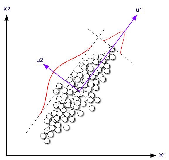
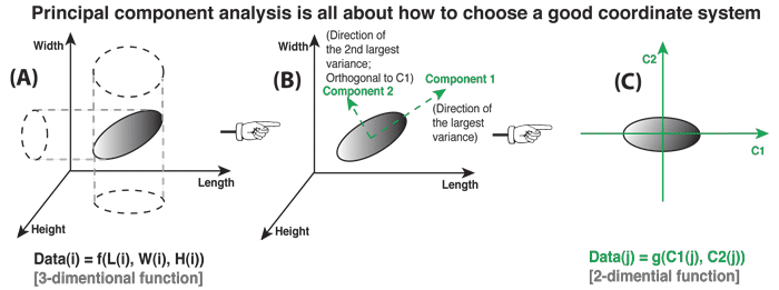
Principal Component Analysis (PCA)
In a nutshell, this is what PCA is all about: Finding the directions of maximum variance in high-dimensional data and project it onto a smaller dimensional subspace while retaining most of the information.
Lab
Load IRIS dataset and plot as points in space (choose a couple features)
Compute SVD of covariance and plot largest singular vectors.
What happens if we don't remove the means properly?
Now how do we look at the data in the "principal directions"?