Unstructured Data & Natural Language Processing

Keith Dillon
Fall 2019

Topic 7: Graph and Spectral Network Methods

This topic:

1. Eigendecomposition review
2. Graphs
3. PageRank
4. Spectral embedding
5. Spectral clustering

Reading:

• "Spectral Theory of Unsigned and Signed Graphs. Applications to Graph Clustering: a Survey" - Jean Gallier www.cis.upenn.edu/~jean/spectral-graph-notes.pdf
• "How Google Ranks Web pages", Brian White, 2004

I. Eigendecompositions

Famous Matrices: Diagonal matrix

$$\mathbf D = \begin{bmatrix} D_{1,1} & 0 & 0\\ 0 & D_{2,2} & 0 \\ 0 & 0 & D_{3,3}\\ \end{bmatrix}$$

Can completely describe with a vector $\mathbf d$ with $d_i = D_{i,i}$

Hence we write "$\mathbf D = \text{diag}(\mathbf d)$" and "$\mathbf d = \text{diag}(\mathbf D)$"

Relate to Hadamard product of vectors $\mathbf D \mathbf v = \mathbf d \odot \mathbf v$.

Famous Matrices: Diagonal matrix - Applications

1. Consider product $\mathbf D \mathbf v$

2. Consider products $\mathbf D \mathbf A$ and $\mathbf A \mathbf D$

3. Consider norm $\Vert \mathbf D \mathbf v \Vert_2$

4. Consider $\mathbf D_1 \mathbf D_2$

5. Consider power $\mathbf D^n$

6. Consider inverse of diagonal matrix $\bf D$

7. Solve linear system $\mathbf A \mathbf x = \mathbf b$ when $\mathbf A$ is diagonal.

Famous Matrices: Orthogonal matrix

Square marix where columns are orthogonal, i.e. $\mathbf a_i^T \mathbf a_j = 0$ when $i \ne j$

Orthonormal matrix $\rightarrow$ also have $\mathbf a_i^T \mathbf a_i = 1$

Famous Matrices: Orthogonal matrix - Applications

Geometrically, orthonormal matrices implement rotations.

Very easy inverse

Solve linear system $\mathbf U \mathbf x = \mathbf b$ for $\mathbf x$ when $\mathbf U$ is orthonormal.

Solve matrix system $\mathbf U \mathbf A = \mathbf V$ for $\mathbf A$ when $\mathbf U$ is orthonormal.

Eigendecomposition

Reconsider: $${\bf A}{\bf u} = \lambda {\bf u}$$

IF $\mathbf A$ is $n \times n$ symmetric and real, we can find $n$ eigenvectors $\{ \mathbf u_i \}$ with corresponding real eigenvalues $\lambda_i$, i.e.

$${\bf A}{\bf u_i} = \lambda_i {\bf u_i}$$

If the eigenvalues are distinct, the eigenvalues are orthogonal. Otherwise they may not be orthogonal but are still linearly independent, so we can make an orthogonal basis.

Write this as ${\bf A}{\bf U} = $ ?

Diagonalization

a.k.a. Eigendecomposition

a.k.a. Spectral Decomposition)

$$ {\bf A}{\bf U} = {\bf U} \boldsymbol\Lambda \rightarrow {\bf A} = {\bf U} \boldsymbol\Lambda {\bf U}^{-1} $$

We can also solve for $\boldsymbol\Lambda$ = ?

Famous Matrices: Normal matrix

A real matrix $\bf A$ is a normal matrix if:

$$ \mathbf A \mathbf A^T = \mathbf A^T \mathbf A$$

Note this must be a square matrix due to matrix multiplication rules.

Examples of Normal matrices:

1. $\mathbf A = \mathbf B \mathbf B^T$ for some $m \times n$ matrix $\bf B$

2. $\mathbf A = \mathbf B^T \mathbf B$ for some $m \times n$ matrix $\bf B$

Famous Matrices: Normal matrix - value

If a real matrix $\bf A$ is a normal matrix then its eigenvectors are orthonormal.

$$ {\bf A}{\bf U} = {\bf U} \boldsymbol\Lambda \rightarrow ? $$

The Singular Value Decomposition (SVD)

Now we are back to talking about general rectangualr matrices, not square, nor symmetric, nor normal, etc.

The SVD of a $m \times n$ matrix $\bf A$ is:

$${\bf A} = {\bf U S V}^T$$

Where $\bf U$ and $\bf V$ are orthonormal matrices and $\bf S$ is a "rectangular diagonal matrix". E.g.

$${\bf S} = \left[ \begin{matrix} s_1 & 0 & \cdots & 0 \\ 0 & s_2 & \cdots & 0 \\ \vdots & \vdots & \ddots & \vdots \\ 0 & 0 & \cdots & s_m \\ \vdots & \vdots & \vdots & \vdots \\ 0 & 0 & \cdots & 0 \end{matrix} \right] \text{, or } {\bf S} = \left[ \begin{matrix} s_1 & 0 & \cdots & 0 & ... & 0 \\ 0 & s_2 & \cdots & 0 & ... & 0\\ \vdots & \vdots & \ddots & \vdots \\ 0 & 0 & \cdots & s_m & ... & 0\\ \end{matrix} \right] $$

$s_i$ are the singular values of $\mathbf A$ and are sorted in decreasing order $s_1 \ge s_2 \ge ... \ge s_r$

The columns of $\bf U$ and $\bf V$ are the left and right singular vectors, respectively.

Exercise: SVD matrix sizes

Using matrix multiplication rules, work out the sizes of each component in the decomposition where $\bf A$ is $m \times n$

$${\bf A} = {\bf U S V}^T$$

.

Draw a picture of what the shapes of the matrices look like.

Hint: orthonormal (and orthogonal) matrices are square.

Relation between SVD and Diagonalization

Now plug ${\bf A} = {\bf U S V}^T$, into the products $\mathbf M_1 = \mathbf A \mathbf A^T$ and $\mathbf M_2 = \mathbf A^T \mathbf A$.

What do you get?

Notice $\mathbf M_1$ and $\mathbf M_2$ are Normal matrices, so write their eigendecompositions.

...Tada! we have discovered a way to compute the SVD using eigenvalue decomposition methods.

Rank (of a matrix $\mathbf A$)

• row-rank = dimension of rowspace
• column-rank = dimension of column space
• Surprise! They're the same.
• Full rank = highest possible rank
• Consider a "full rank" square matrix. What is its nullity?
• Consider a "full rank" $m \times n$ (rectangular) matrix. What is its rank?

The Rank-Nullity theorem (of a $m \times n$ matrix $\mathbf A$)

Nullity defined as dimension of nullspace.

$$ Rank(\mathbf A) + Nullity(\mathbf A) = n $$

Note that while rank is a "symmetric" concept, nullspace is specific to left or right.

SVD and rank

The rank of a matrix is the number of nonzero singular values it has.

However in practice, hard zeros are rare. How would we deal with having tiny values which should be zeros?

Covariance matrix versus Normal matrices

Consider how we can compute variances and covariances using a matrix product.

In many applications we need to center the data matrix by subtracting the mean from all the data points, called "Mean-deviation Form"

$${\bf \hat{x}}_i = {\bf x}_i - {\bf \mu}$$

This gives us a new data matrix

$${\bf Z} = \left[ \begin{matrix} {\bf \hat{x}}_1^T \\ \vdots \\ {\bf \hat{x}}_n^T \end{matrix} \right] = \left[ \begin{matrix} ({\bf x}_1 - {\bf \mu})^T \\ \vdots \\ ({\bf x}_n - {\bf \mu})^T \end{matrix} \right] = \left[ \begin{matrix} x_{11} - \mu_1 & \cdots & x_{1d} - \mu_d \\ \vdots & \ddots & \vdots \\ x_{n1} - \mu_1 & \cdots & x_{nd} - \mu_d \end{matrix} \right]$$

$\bf Z$ is called centered data matrix for mean-deviation form, because $mean({\bf Z}) = {\bf 0}$, that is the mean coincides with the origin of the data space.

Covariance Matrix

The covariance matrix is a $d \times d$ symmetric matrix that gives the covariance for each pair of attributes

$${\bf \Sigma} = \left[ \begin{matrix} \sigma_1^2 & \sigma_{12} & \cdots & \sigma_{1d} \\ \sigma_{21} & \sigma_2^2 & \cdots & \sigma_{2d} \\ \vdots & \vdots & \ddots & \vdots \\ \sigma_{d1}^2 & \sigma_{d2} & \cdots & \sigma_d^2 \end{matrix} \right]$$

The diagonal elements $\sigma_j^2$ specity the variance of $j$th attribute or column of $\bf D$, whereas the off-diagonal elements $\sigma_{jk} = \sigma_{kj}$ represent the covariance between pairs of columns.

$$\sigma_j^2 = \frac{1}{n} \sum_{i=1}^n (x_{ij} - \mu_j)^2$$$$\sigma_{jk} = \frac{1}{n} \sum_{i=1}^n (x_{ij} - \mu_j)(x_{ik} - \mu_k)$$

Covariance Matrix

If we represent columns of $\bf Z$ with $n$-dimensional vector ${\bf z}_j$:

$${\bf z}_j = \left[ \begin{matrix} x_{1j} - \mu_j \\ \vdots \\ x_{nj} - \mu_j \end{matrix} \right]$$

then we can write variances in a compact form:

$$\sigma_j^2 = \frac{1}{n} {\bf z}_j^T {\bf z}_j~~~~~\text{and}~~~~~\sigma_{jk} = \frac{1}{n} {\bf z}_j^T {\bf z}_k$$

The covariance matrix can be written in a compact form using the centered data matrix as

$${\bf \Sigma} = \frac{1}{n} {\bf Z}^T {\bf Z}$$

This is often called the scatter matrix.

II. Introduction to Graphs

Graphs

$$G = (V,E)$$

1. A set of Nodes $V=\{v_1, ..., v_n\}$
2. A set of Edges $E = \{e_1, ..., e_m\}, e_i \in V\times V $ - either binary (there or not there) or weighted, between pairs of nodes

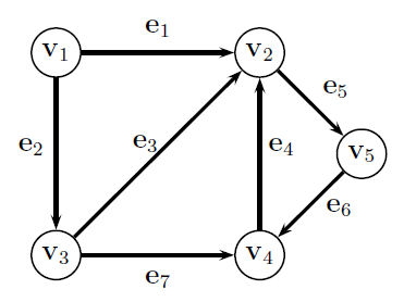
Degree

Node Degree - $d(v_i)$ number of edges entering or leaving node $v_i$ = In_degree + out_degree

Degree Matrix - diagonal matrix of node degrees

$$\mathbf D = \begin{bmatrix} d_{1} & 0 & 0 & 0 & 0\\ 0 & d_{2} & 0 & 0 & 0\\ 0 & 0 & d_{3} & 0 & 0\\ 0 & 0 & 0 & d_{4} & 0\\ 0 & 0 & 0 & 0 & d_{5} \end{bmatrix} = \begin{bmatrix} 2 & 0 & 0 & 0 & 0\\ 0 & 4 & 0 & 0 & 0\\ 0 & 0 & 3 & 0 & 0\\ 0 & 0 & 0 & 3 & 0\\ 0 & 0 & 0 & 0 & 2 \end{bmatrix} $$

Adjacency Matrix

an $n\times n$ matrix $\mathbf A$ where...

• $A_{i,j}=+1$ if there is an edge from nodes $i$ to $j$
• $A_{j,i}=+1$ if there is an edge from nodes $j$ to $i$

Treats all types of graphs the same

$$\mathbf A = \begin{bmatrix} 0 & 1 & 1 & 0 & 0\\ 1 & 0 & 1 & 1 & 1\\ 1 & 1 & 0 & 1 & 0\\ 0 & 1 & 1 & 0 & 1\\ 0 & 1 & 0 & 1 & 0 \end{bmatrix} $$

Adjacency Matrix - Variants

1. Signed
2. Directed
3. Weighted (often called $\mathbf W$)

Also can have any combination of these properties.

Network methods overwhelmingly focus on unsigned, undirected, binary case. Weighted version also common.

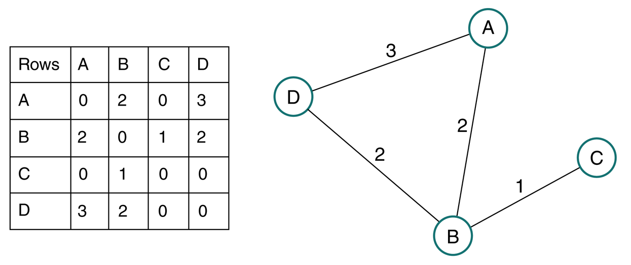
Weighted graph

Generally define weight matrix $\mathbf W$ as weighted analog to adjacency matrix, since also can define a binary adjacency matrix for same graph.

Degree of node in weighted graph is sum of weights of edges connecting node

Degree vector $\mathbf d = \mathbf W \mathbf 1$

Degree matrix $\mathbf D = \text{diag}(\mathbf d)$

Adjacency matrix interpretation

Diffusion operator - applying $\mathbf A$ to vector of values at nodes results in values at neighboring nodes.

Eigenvector intuition - consider what it means, therefore, if $\mathbf A \mathbf x = \lambda \mathbf x$

Using Covariance matrix as a Weighted adjacency matrix

Recall we could equivalently use the (first) eigenvectors of $\mathbf L_{rw}$ or the (last) eigenvectors of $\mathbf W$.

Consider the choice $\mathbf W = \mathbf C = \mathbf X \mathbf X^T$

What is $W_{ij}$ in terms of data samples?

How do the eigenvectors of $\mathbf W$ relate to singular vectors of $\mathbf X$?

NetworkX Example

https://networkx.github.io/documentation/stable/tutorial.html https://networkx.github.io/documentation/stable/reference/generated/networkx.convert_matrix.from_numpy_matrix.html

import matplotlib.pyplot as plt
import networkx as nx
import numpy as np

A = np.random.rand(5,5)
A = A*(A>0.5)
G = nx.from_numpy_matrix(np.matrix(A), create_using=nx.DiGraph)
layout = nx.spring_layout(G)
nx.draw(G, layout)
#nx.draw_networkx_edge_labels(G, pos=layout)
nx.draw_networkx_labels(G, pos=layout)
plt.show();

Breast Cancer Data example

from sklearn import datasets
dat = datasets.load_breast_cancer()

Covariance Matrix from features

plt.imshow(C)
plt.colorbar();

Graph using large covariances as edges

Covariance of Features for Malignant tumors

network0()

Covariance of Features for Benign tumors

network0()

II. PageRank

Recall: Scoring Function

Choose document to Maximize $score(query,document)$

• PageRank - Weight document (webpages) matches based on network connectivity
  1. find set of documents which match query
  2. rank based on "authority" as determined by links to document
     • To solve "tyranny of TF scores" (term-frequencies, used as weighting previously).
     • e.g. query = "CNN", presumably "cnn.com" is the search result with the most authority, though other results may use the word more because cnn.com may not talk about CNN very much, but instead the changing news itself. Meanwhile "ihatecnn.com" will mention CNN constantly as it obsesses over CNN's mistakes.
• HITS (Hyperlink-Induced Topic Search)
  1. find set of documents which match query
  2. rank based on authority within set of matches only

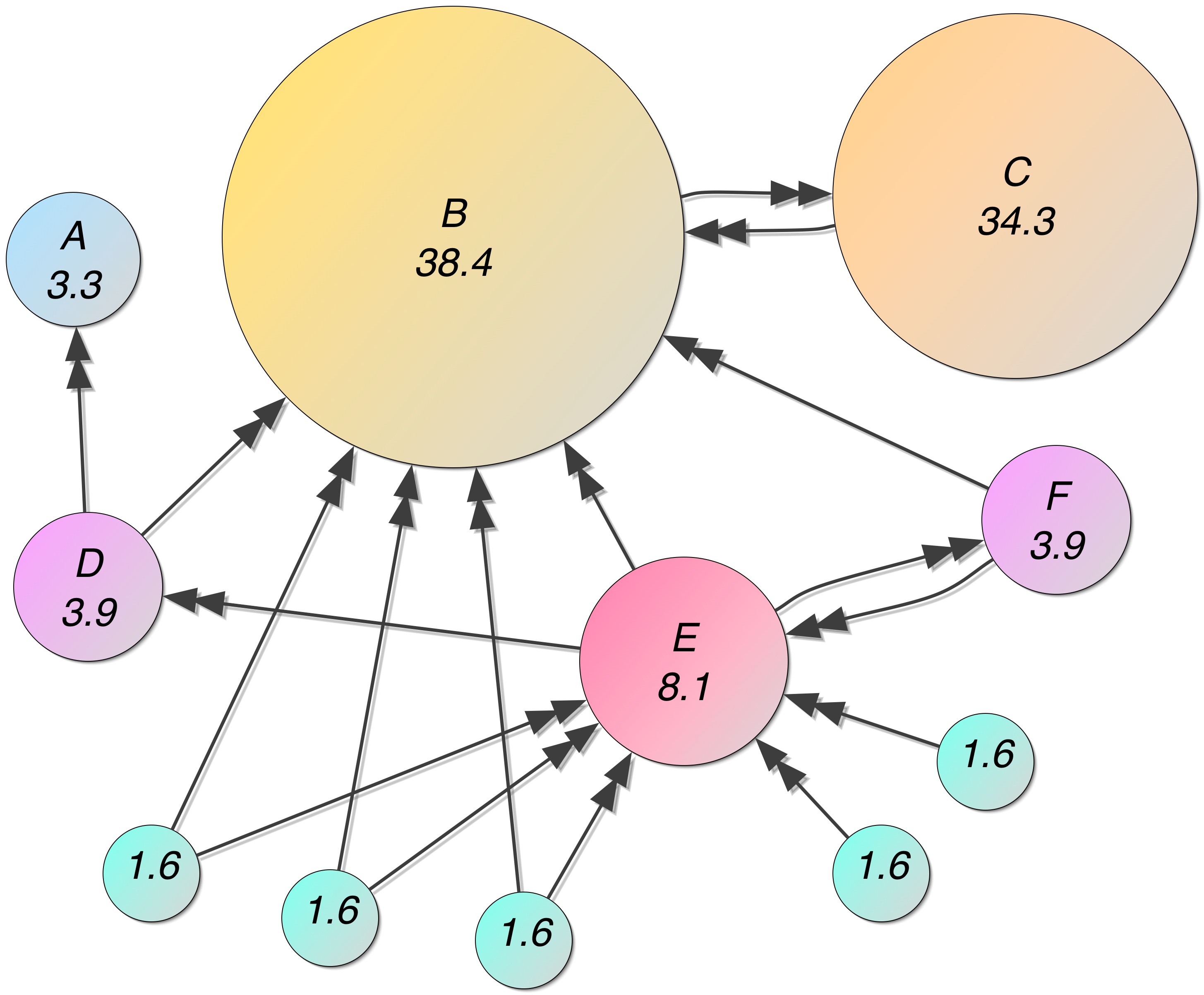
PageRank: setup

We want to rank search results based on website "importance".

"Very simple method": create adjacency matrix of links. Weight pages by in-degree. Node "value" vector...

$$ \bb v = \bb A \bb 1$$

Improvement #1

Downweight incoming edge by outdegree of node it comes from, $\bb n = \bb A^T \bb 1$

$$P_{ij}=\frac{A_{ij}}{n_{j}}$$$$ \bb v = \bb P \bb 1$$

Improvement #2

Up-weight incoming edge by importance of node it comes from

$$ \bb v = \bb P \bb v$$

And we have an eigenvector problem.

So find the eigenvalue of the internet to rank its web pages.

Final improvement: Teleportation

• zero out-degree nodes, groups of nodes
• solve by treating every node as having very weak connections to all other nodes.
• web surfer just randomly goes to a new page and starts surfing again

$$ \bb Q = r\bb P + (1-r) \bb T$$

• $\bb T$ = teleportation matrix, $T_{ij} = \frac{1}{N}$.
• $0<r<1$, Google uses $r=0.85$.

Example from wikipedia...

III. Spectral Embedding & Clustering

Graph Laplacians

Unnormalized - binary graphs: $ \mathbf L = \mathbf D - \mathbf A $, weighted graphs: $ \mathbf L = \mathbf D - \mathbf W $

Symmetric: $ \mathbf L_{sym} = \mathbf D^{-\frac{1}{2}} \mathbf L \mathbf D^{-\frac{1}{2}} $

Random walk: $ \mathbf L_{rw} = \mathbf D^{-1} \mathbf L $

Spectral Graph Drawing (a.k.a. Embedding)

The drawing of a graph is a function $\boldsymbol\rho(\cdot)$ which assigns a point in space $\boldsymbol\rho(v_i)$ to each node $v_i$

The matrix $\mathbf R$ of a graph drawing is a $m\times n$ matrix whos $i$th row is $\boldsymbol\rho(v_i)$

Energy of a drawing

View edges as springs and our goal is to make a graph with minimum energy stored in the springs

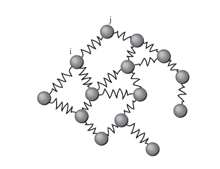
Weight of edge is strength of spring

\begin{align} \varepsilon(R) &= \sum_{\text{edges} \;i\leftrightarrow j} w_{ij} \Vert\boldsymbol\rho(v_i) -\boldsymbol\rho(v_j)\Vert^2 \\ &= \text{trace}(\mathbf R^T \mathbf L \mathbf R) \end{align}

So a high edge weight means the nodes want to be close together

Balanced Orthogonal Drawing

Representation is balanced if $\mathbf 1^T \mathbf R = \mathbf 0^T$ - sum of columns is zero

To prevent trivial solutions (e.g. all nodes placed at the origin) we add the constraint that $\mathbf R$ is an orthogonal matrix, i.e. $\mathbf R^T \mathbf R = \mathbf I$

Minimum Energy Balanced Orthogonal Drawing

For a weighted Graph Laplacian $\mathbf L$

with eigenvalues $0=\lambda_1<\lambda_2\le \lambda_3 \le... \le \lambda_m$

The Minimum Energy Balanced Orthogonal Drawing has energy $\lambda_2+...+\lambda_{n+1}$ (where $n<m$).

The representation $\mathbf R$ consisting of the associated unit eigenvectors $u_2,...,u_{n+1}$ achieves this minimum energy.

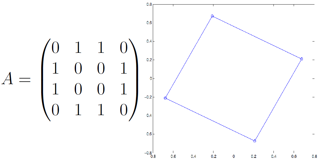
2D Case

1. Compute 2nd and 3rd eigenvectors $\mathbf u_2$ and $\mathbf u_3$, i.e. corresponding to two smallest nonzero eigenvalues
2. Form $m\times 2$ representation matrix $\mathbf R = (\mathbf u_2, \mathbf u_3)$ with eigenvectors as columns
3. Place node $v_i$ at point defined by $i$th row of $\mathbf R$

Example

Network Embedding versus "Data Embedding"

Note when dealing with network methods we have two possible starting points:

1. Starting with an already-made network (given an adjacency matrix describing connections between a set of nodes)
2. Starting with a dataset (given a matrix of samples versus features), where the first step is to form the network (somehow)

In #2, we start with a set of sample vectors, then compute a bunch of embedded model locations, which might be viewed as new sample vectors (now in a lower number of dimensions).

What are other names used for approach #2?

Graph cut

Starting with a graph $G=(V,E)$

We choose a subset of nodes $U \subset V$, where $\bar{U}$ is the set of nodes in $V$ that are not in $U$

$$ \text{cut}(U) \equiv \sum_{v_i\in U, v_j\in \bar{U}} w_{ij} $$

The sum of weights of edges we would cut to remove $U$ from $V$

Multiple cluster version ($K$ = # clusters)

$$ \text{cut}(U_1,...U_K) \equiv \frac{1}{2} \sum_{i} \text{cut}(U_i) $$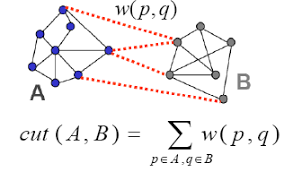

Mincut problem

Choose subset $U^*$ that minimizes cut: $$ \arg\min_U \text{cut}(U) $$

• Describe subset(s) with a class vector $\mathbf c$
• For $K=2$, have $c_i\in \{0,1\}$
• For general $K$, have $c_i\in [0,1,...,K]$

For $K=2$ can be solved efficiently, however algorithms which minimize the cut often end up with a trivial solution which chooses a subset consisting of a single node.

This is addressed by changing the problem to make these trivial solutions less likely. For example by weighting the objective by the size of the subset (so smaller subsets are less desirable).

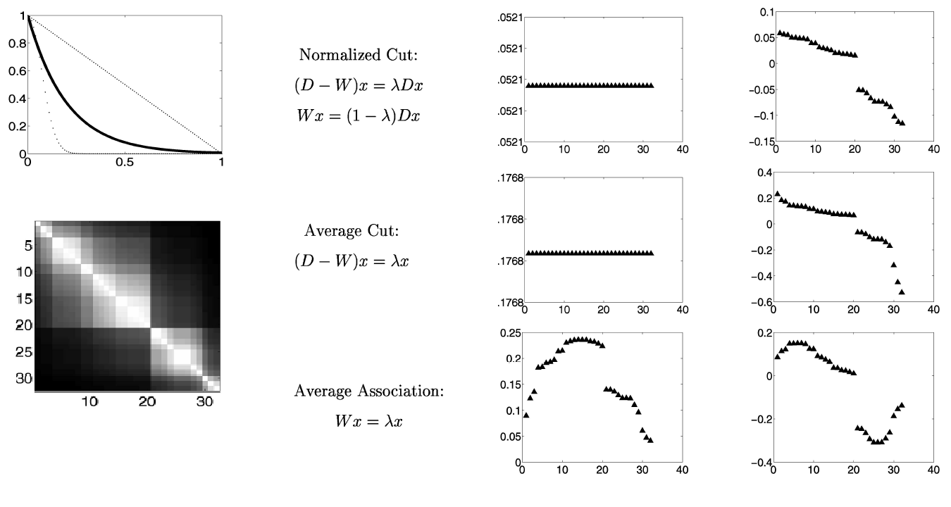
Normalized cut

$$ \text{NCut}(U_1,...,U_K) \equiv \sum_{i} \frac{\text{Cut}(U_i,\bar{U}_i)}{\text{Vol}(U_i)} $$

NP-hard optimization problem: $$ \arg\min_{U_1,...,U_K} \text{NCut}(U_1,...,U_K) $$

Spectral Clustering

Continuous relaxation of class membership. Instead of $c_i\in [0,1,...,K]$, allow continuous values for $c_i$. Then choose class based on nearest integers.

$K=2$ case: Jianbo Shi and Jitendra Malik. "Normalized cuts and image segmentation". Transactions on Pattern Analysis and Machine Intelligence, 22(8):888-905, 2000.

$K>2$ case: Stella X. Yu. "Computational Models of Perceptual Organization". PhD thesis, Carnegie Mellon University, 2003 Dissertation; Stella X. Yu and Jianbo Shi. "Multiclass spectral clustering". In 9th International Conference on Computer Vision, IEEE, 2003.

Spectral Clustering, $K=2$ (Shi and Malik)

1. Given an image or image sequence, set up a weighted graph $G = (V,E)$ and set the weight on the edge connecting two nodes to be a measure of the similarity between the two nodes.
2. Solve $\mathbf L_{sym}\mathbf x = \lambda \mathbf x$ for eigenvectors with the smallest eigenvalues.
3. Use the eigenvector with the second smallest eigenvalue to bipartition the graph.
4. Decide if the current partition should be subdivided and recursively repartition the segmented parts if necessary.

Shi and Malik. "Normalized cuts and image segmentation". Transactions on Pattern Analysis and Machine Intelligence, 22(8):888-905, 2000.

Spectral Clustering, $K>2$ (Ng, Jordan, & Weiss)

Given a set of points $S = \{\mathbf s_1, ... , \mathbf s_n\}$ with $\mathbf s_i \in \mathbf R^n$ that we want to cluster into $k$ subsets

1. Form the affinity matrix defined by $A_{ij} = \exp(-\frac{1}2\sigma\Vert \mathbf s_i - \mathbf s_j\Vert^2)$ if $i \ne j$ , and $A_{ii} = 0$.
2. Define $\mathbf D$ to be the diagonal matrix whose $(i, i)$-element is the sum of $\mathbf A$'s $i$th row, and construct the matrix $\mathbf L = \mathbf D^{-\frac{l}{2}} \mathbf A \mathbf D^{-\frac{l}{2}}$
3. Find $\mathbf x_1, \mathbf x_2, ..., \mathbf x_k$ , the $k$ largest eigenvectors of $\mathbf L$ (chosen to be orthogonal to each other in the case of repeated eigenvalues), and form the matrix $\mathbf X = (\mathbf x_1, \mathbf x_2, ..., \mathbf x_k)$ by stacking the eigenvectors in columns.
4. Form the matrix $\mathbf Y$ from $\mathbf X$ by renormalizing each of $\mathbf X$'s rows to have unit length (i.e. $Y_{ij} = [\sum_j X_{ij}]^{-\frac{1}{2}} X_{ij}$).
5. Treating each row of $\mathbf Y$ as a point in $\mathbf R^k$ , cluster them into $k$ clusters via $K$-means or any other algorithm (that attempts to minimize distortion).
6. Finally, assign the original point $\mathbf s_i$ to cluster $j$ if and only if row $i$ of the matrix $\mathbf Y$ was assigned to cluster $j$.

Ng, Jordan, Weiss, "On spectral clustering: Analysis and an algorithm" Advances in neural information processing, 2002.

Eigenvector Variants

• First one is random walk Laplacian
• Equivalent to using normalized version of weight matrix (unit row sums).

Recap

Assume we start with a dataset and need to form the network to apply spectral graph methods.

Given matrix of data $\mathbf X$ where rows are samples and columns are features

1. Form either a weighted adjacency matrix $\mathbf W$ or a binary adjacency matrix $\mathbf A$ via some approach that quantifies similarity between samples.

• Simple approach: take inner product $\mathbf x_i^T \mathbf x_j$ between two samples $\mathbf x_i$ and $\mathbf x_j$ and this as $W_{ij}$ or perhaps use some function of this value such as $|\mathbf x_i^T \mathbf x_j|$.

1. Compute Laplacian of network such as $\mathbf L = \mathbf D - \mathbf W$ or some other version.

2. Compute eigenvectors $\mathbf u_1, ..., \mathbf u_k$ for $k$ smallest eigenvalues of $\mathbf L$,

3. Discard $\mathbf u_1$ and form matrix $\mathbf U$ with $\mathbf u_2, ..., \mathbf u_k$ as columns.

4. Use rows of $\mathbf U$ as embedded samples.

5. Cluster these embedded samples to perform partitioning of graph and therefore of original samples.

Caveat Roundup

• We also assumed the graph makes a single connected component. If we are automatically generating a big sparse graph from a dataset, this assumption may be violated. In general, for a non-negative weighted graph the first eigenvalue (which takes value 0 and has eigenvector $\mathbf 1$) will have multiplicity equal to the number of connected compoennts. Discard all of these trivial eigenvectors.
• For the clustering problem, the choise of clusters $k$ is an open problem (as usual with clustering methods).

• We have lots of (vaguely-similar) options for how to compute similarity and therefore the choice of $\mathbf W$ or $\mathbf A$
• We have a few (also vaguely-similar) options for choice of Laplacian (unnormalized, symmetric, random walk), and a few more variants depending on less-common kinds of networks (signed, directed)

Don't feel overwhelmed by all these variants. They lead to largely-similar results, though some will work better than others for your problem. For example, thresholding of similarities to use a binary adjacency matrix rather than weighted might make the results a bit more robust vs noise, or less so, depending on the data