Unstructured Data & Natural Language Processing
Keith Dillon
Fall 2019
Topic 8: Gaussian Graphical Models
I. Gaussian Review
1-D Recap
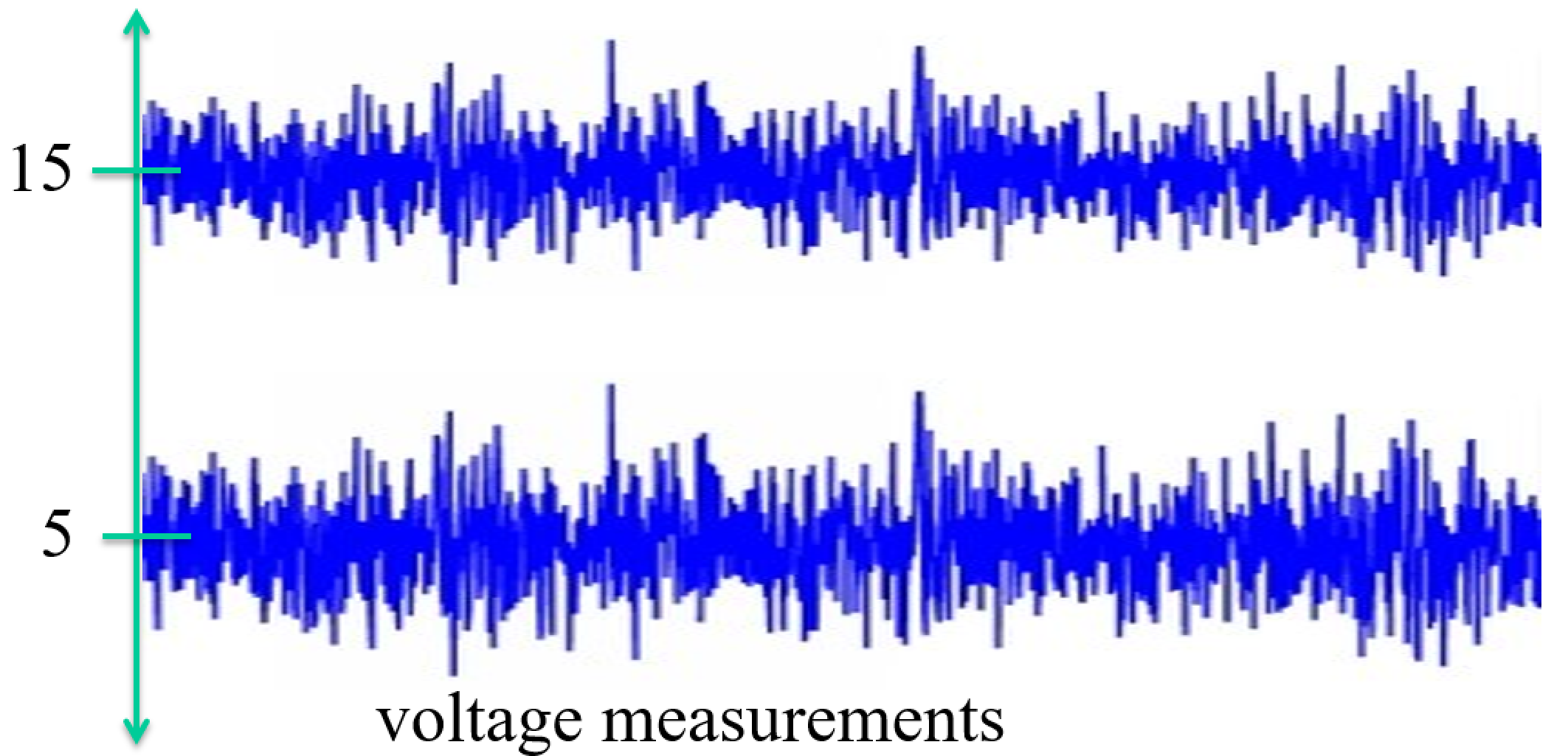
\begin{align} \text{Population mean} &= \mu = \frac{\sum_{i=1}^N x_i}{N} \\ \text{Sample mean} &= \bar{x} = \frac{\sum_{i=1}^n x_i}{n} \\ \text{Population variance} &= \sigma^2 = \frac{\sum_{i=1}^N (x_i - \mu)^2}{N} \\ \text{Sample variance} &= s^2 = \frac{\sum_{i=1}^n (x_i - \bar{x})^2}{n - 1} = \frac{\sum_{i=1}^n x_i^2 - \frac{1}{n}(\sum_{i=1}^n x_i)^2}{n - 1} \\ \text{Standard deviation} &= \sqrt{\text{Variance}} \end{align}Review: Normal a.k.a. Gaussian Distribution $X \sim N(\mu, \sigma) = G(\mu, \sigma)$
$$ f(x) = \frac{1}{\sigma \sqrt{2 \pi}} exp \left(- \frac{(x - \mu)^2}{2 \sigma^2} \right) \text{, for } x \in R $$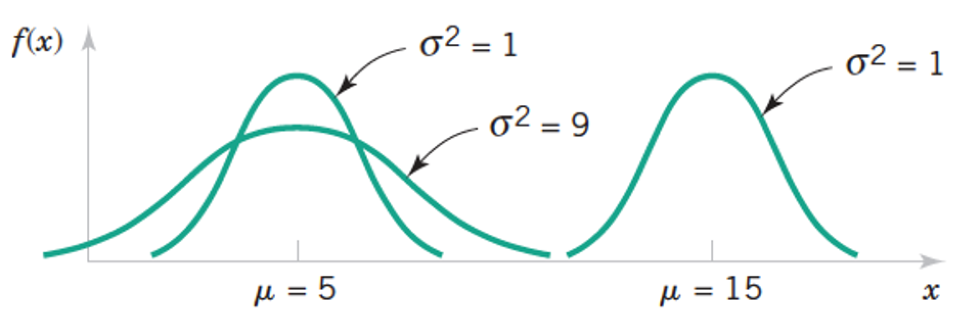
import numpy as np
from matplotlib import pyplot as plt

def univariate_normal(x, mean, var):
    return ((1. / np.sqrt(2 * np.pi * var)) * np.exp(-(x - mean)**2 / (2 * var)))

x = np.linspace(-5,5,1000)
plt.plot(x,univariate_normal(x,1,2));
plt.show()

Review: Joint Distributions
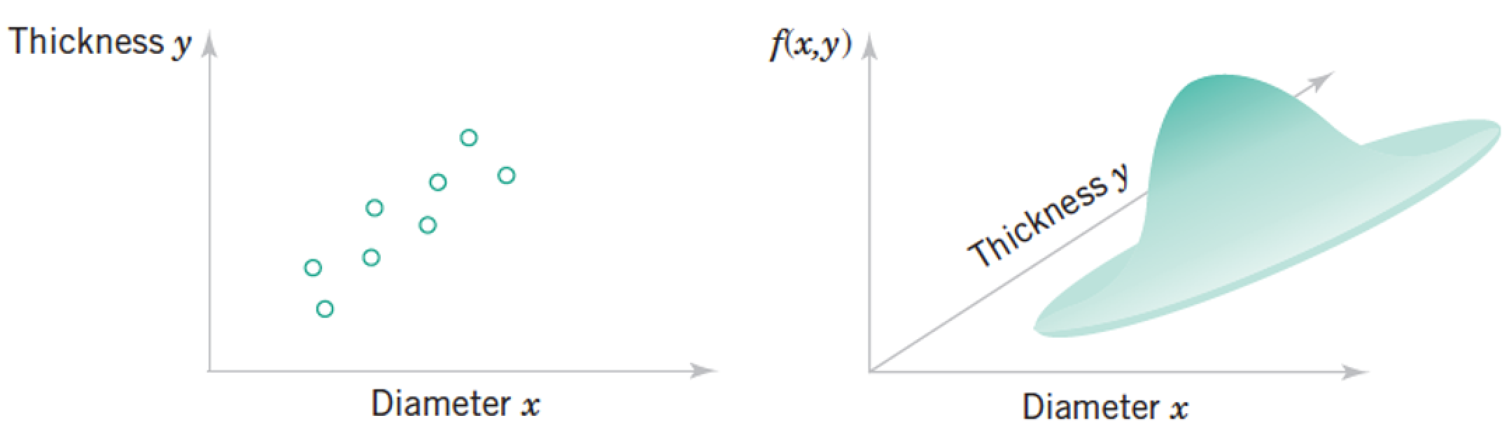
Each "sample" as a list of features, which we model as a vector of random variables, $ \mathbf x = \begin{pmatrix} Diameter \ Thickness
\end{pmatrix}
\begin{pmatrix} x_1 \\ \vdots \\ x_n \\ \end{pmatrix}$
Each point in the distribution is simultanous probability of all the features taking the particular vector of numbers at the point.
Multivariate Data - describing relationships
"Multivariate" dataset ~ a matrix with samples for rows and features for columns. Each column (a.k.a. feature) is also known as a variable.
Just focusing on two variables for the moment, say column1 = $x$, and column2 = $y$.
Correlation(s)
\begin{align} \text{Variance} &= s^2 = \frac{\sum_{i=1}^n (x_i - \bar{x})^2}{n - 1} = \frac{\sum_{i=1}^n x_i^2 - \frac{1}{n}(\sum_{i=1}^n x_i)^2}{n - 1} \\ \text{Standard deviation} &= \sqrt{\text{Variance}} \end{align}\begin{align} \text{Correlation Coefficient} &= r = \frac{ \sum_{i=1}^n (x_i - \bar{x})(y_i - \bar{y})}{\sqrt{\sum_{i=1}^n(x_i - \bar{x})^2}\sqrt{\sum_{i=1}^n(y_i - \bar{y})^2}} = \frac{S_{xy}}{\sqrt{S_{xx} S_{yy}}} \\ %\text{''Corrected Correlation''} % &= S_{xy} = \sum_{i=1}^n (x_i - \bar{x})(y_i - \bar{y}) % = \sum_{i=1}^n x_i y_i - \frac{1}{n}(\sum_{i=1}^n x_i)(\sum_{i=1}^n y_i) \\ \text{Covariance} &= S_{xy} = \frac{1}{n-1}\sum_{i=1}^n (x_i - \bar{x})(y_i - \bar{y}) % = \sum_{i=1}^n x_i y_i - \frac{1}{n}(\sum_{i=1}^n x_i)(\sum_{i=1}^n y_i) \end{align}Look kind of familiar? Relate to variance. Note $"Cov(x,x)" = S_{xx}= \sigma_x^2$.
Questions
What are $S_{xx}$ and $S_{yy}$ also called?
Can you relate the covariance to a distance metric?
Exercises
\begin{align} \text{Correlation Coefficient} &= r = \frac{ \sum_{i=1}^n (x_i - \bar{x})(y_i - \bar{y})}{\sqrt{\sum_{i=1}^n(x_i - \bar{x})^2}\sqrt{\sum_{i=1}^n(x_i - \bar{x})^2}} = \frac{S_{xy}}{\sqrt{S_{xx} S_{yy}}} \end{align}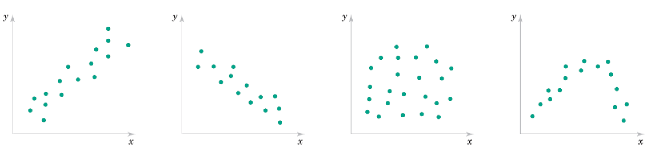
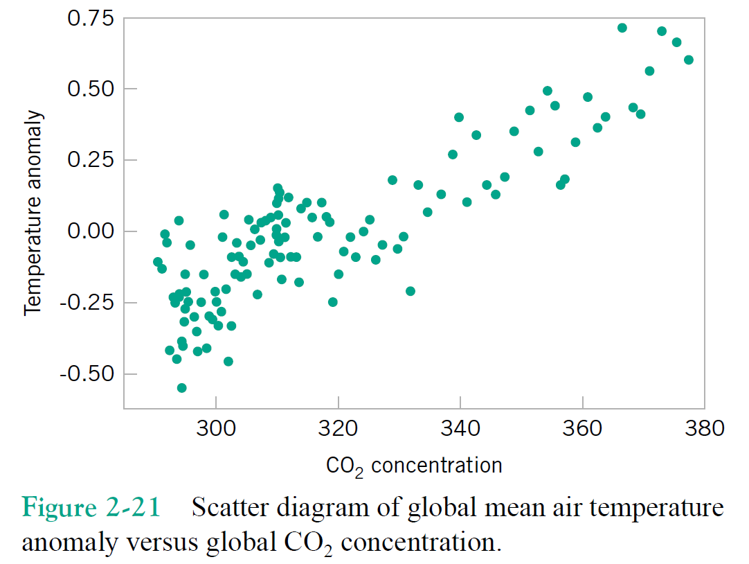
Roughly what are the correlation coefficients here?

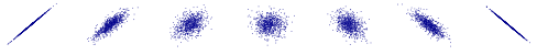
Correlation Qualitative Behavior
- What does magnitude tell you about the relationship?
- What does sign tell you about the relationship?
- Would you expect the Covariance to be similar?
Multivariate Gaussian (for $n$ dimensions)
$$ f(\mathbf x) = \frac{1}{ \sqrt{2 \pi^n |\boldsymbol\Sigma|}} \exp \left(- \frac{1}{2} (\mathbf x - \boldsymbol \mu)^T \boldsymbol\Sigma^{-1} (\mathbf x - \boldsymbol \mu) \right) \text{, for } \mathbf x \in R^n $$- Mean vector as centroid of distribution
- Covariance matrix describes spread - correlations between variables $\Sigma_{ij} = S_{\mathbf x_i \mathbf x_j}$
...Terminology note...
In general terms, covariance is a kind of metric for correlation.
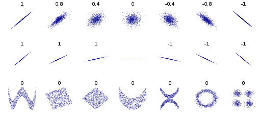
Formal definition of correlation (i.e. Pearson) differs from covariance only in scaling, so that it ranges between $\pm 1$ rather than some max and min.
I will tend to use them interchangeably, where correlation means the more intuitive concept and covariance the formal matrix we compute (or its elements).
def multivariate_normal(x, n, mean, cov):
    return (1./(np.sqrt((2*np.pi)**n * np.linalg.det(cov))) * np.exp(-1/2*(x - mean).T@np.linalg.inv(cov)@(x - mean)))


mean = np.array([35,70])
cov = 100*np.array([[1,.5],[.5,1]])
pic = np.zeros((100,100))
for x1 in np.arange(0,100):
    for x2 in np.arange(0,100):
        x = [x1,x2]
        pic[x1,x2] = multivariate_normal(x, 2, mean, cov)

plt.contour(pic);

cov
np.linalg.inv(cov)
Exercise: independence of random variables
$$P(x_1,x_2) = P(x_1)P(x_2)$$What does this mean for a multivariate Gaussian distribution?
Using Covariance matrix as a Weighted adjacency matrix
Recall we could equivalently use the (first) eigenvectors of $\mathbf L_{rw}$ or the (last) eigenvectors of $\mathbf W$.
Consider the choice $\mathbf W = \mathbf C = \mathbf X \mathbf X^T$
What is $W_{ij}$ in terms of data samples?
How do the eigenvectors of $\mathbf W$ relate to singular vectors of $\mathbf X$?
Multivariate Gaussians as Networks
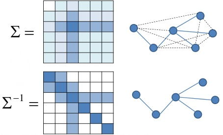
Recall use of covariance matrix as way to define network, covariances for similarities between variables
In this case, can view entire network as a description of a multivariate Gaussian distribution
- nodes represent random variables
- edges represent dependencies between random variables, nonzero off-diagonal terms in the covariance matrix
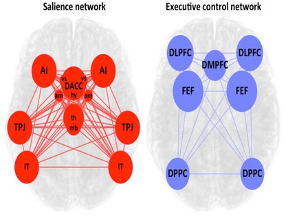
Example: brain networks inferred by measuring pairwise correlations between different regions
Note the sample covariance matrix is only an estimate of the true covariance between random variables. And in general the covariance between samples of data will never be zero. So we may choose to threshold small values in the covariance matrix. Or perhaps use more sophisticated means to find a sparse covariance matrix given data. The problem of finding better estimates is called covariance estimation.
Also note that it doesn't make too much sense to say that a pair of random variables are dependent on a third variable, but somehow independent of each other. Everything will tend to look connected to everything else.
Covariance Estimation
The problem of estimating a valid covariance matrix from data
Methods we know: computing sample covariances.
Network-inspired idea: compute sample covariance and set small values to zero for making s spase network.
Problem #1: will these estimates be invertible? (as we need to describe the Gaussian)
Problem with using Correlations for network edges
Pretty much everything will have some degree of correlation with everything else.
Consider a sequence of words with the bigram assumption. Distant words are still correlated even though they are conditionally independent.
Conditional Correlation
a.k.a. partial correlation $\rho_{xy\cdot z}$
The correlation between $x$ and $y$ controlling for z
II. Gaussian Graphical Models
Precision and Precision Matrix
The Precision of a variable is commonly (though not always) deined as the inverse of the variance. $p = \sigma^{-2}$.
Higher spread means higher variance and hence lower precision.
The Precision Matrix is the inverse of the Covariance matrix. $\mathbf P = \boldsymbol\Sigma^{-1}$.
This matrix is used in the multivariate Gaussian.
Gaussian graphical models
Recall from Bayesian networks that correlation does not imply causation.
It is much more interesting to describe the conditional correlation (a.k.a. partial correlation) between variables, rather than simply the correlation.
If conditional correlation is zero, the variables are conditionally independent.
Amazingly, partial correlations are closely-related to the inverse of the covariance matrix, $\mathbf\Sigma^{-1}$, also called the precision matrix.
Also known as Gauss Markov Random Fields
Partial correlation and precision matrix
The partial correlation between a pair of variables, conditioned on all the rest, is related (within a scalar) to the $(i,j)$th element of the precision matrix.
\begin{align} \rho_{i,j} = -\frac{\sigma^{i,j}}{\sqrt{\sigma^{i,i}\sigma^{j,j}}} \end{align}Hence a pair of variables $x_i$ and $x_j$ are conditionally independent if $\sigma^{(i,j)}=0$.
Value of zeros in precision matrix
A zero implies conditional independence for a variety of non-Gaussian cases also
Recap
We start by considering a set of random variables $\{x_1, ..., x_m\}$
In practice we will use a vector of samples of each of the random variables $\{\mathbf x_1, ..., \mathbf x_m\}$
We like to create a matrix of data $\mathbf X$ from the vectors, where rows are samples and columns are features
If we subtract the means from each row, we can compute a sample covariance matrix $\mathbf C = \frac{1}{N-1} \mathbf X \mathbf X^T$. (often we ignore the scalar term).
If $\mathbf C$ is invertible, we can estimate the precision matrix $P = \mathbf C^{-1}$.
Nonzero elements of the precision matrix $\sigma^{i,j}$ give edges in the graphical model.
However generally hard zeros don't occur in real data calculations. Instead of thresholding the covariance matrix to make a sparse network, we can threshold the precision matrix.
Graphical Lasso
Instead of thresholding the precision matrix values, we can seek a sparse (approximate) inverse to $\mathbf C$
\begin{align} f(\mathbf x) &= \frac{1}{ \sqrt{2 \pi^n |\boldsymbol\Sigma|}} \exp \left(- \frac{1}{2} (\mathbf x - \boldsymbol \mu)^T \boldsymbol\Sigma^{-1} (\mathbf x - \boldsymbol \mu) \right) \\ &= \frac{\sqrt{|\boldsymbol\Omega|}}{ \sqrt{2 \pi^n }} \exp \left(- \frac{1}{2} (\mathbf x - \boldsymbol \mu)^T \boldsymbol\Omega (\mathbf x - \boldsymbol \mu) \right) \\ &= \frac{\sqrt{|\boldsymbol\Omega|}}{ \sqrt{2 \pi^n }} \exp \left(- \frac{1}{2} \text{trace}(\mathbf S \boldsymbol\Omega)\right) \end{align}Where now $\mathbf S$ is the sample covariance matrix and $\boldsymbol\Omega$ is the precision matrix (whice we view as approximations to $\boldsymbol\Sigma$ and $\boldsymbol\Sigma^{-1}$, respectively)
Graphical Lasso - continued
Now we view $\boldsymbol\Omega$ as the random variable and $\mathbf S$ as the data, so we have the likelihood
\begin{align} P(\mathbf S|\boldsymbol\Omega) = f(\mathbf x) = &= \frac{\sqrt{|\boldsymbol\Omega|}}{ \sqrt{2 \pi^n }} \exp \left(- \frac{1}{2} \text{trace}(\mathbf S \boldsymbol\Omega)\right) \end{align}We wish to compute a sparse estimate for $\boldsymbol\Omega$ so use the prior $p(\lambda\boldsymbol\Omega) \propto \exp(\Vert\boldsymbol\Omega\Vert_1)$ and Bayes law to compute
\begin{align} P(\boldsymbol\Omega |\mathbf S) &= \frac{P(\mathbf S|\boldsymbol\Omega) P(\boldsymbol\Omega)}{P(\mathbf S)} \end{align}The maximum likelihood solution, subject to a constraint that $\boldsymbol\Omega$ has non-negative eigenvalues (hence is a legitimate precision matrix):
\begin{align} \arg\max_{\boldsymbol\Omega \succeq 0} P(\boldsymbol\Omega |\mathbf S) &= \arg\max_{\boldsymbol\Omega \succeq 0} \frac{P(\mathbf S|\boldsymbol\Omega) P(\boldsymbol\Omega)}{P(\mathbf S)} \\ &= \arg\max_{\boldsymbol\Omega \succeq 0} P(\mathbf S|\boldsymbol\Omega) P(\boldsymbol\Omega) \\ &= \arg\max_{\boldsymbol\Omega \succeq 0} \log\{ P(\mathbf S|\boldsymbol\Omega) P(\boldsymbol\Omega) \} \\ &= \arg\max_{\boldsymbol\Omega \succeq 0} \{ \log|\boldsymbol\Omega| - \text{trace}(\mathbf S \boldsymbol\Omega) - \lambda\Vert\boldsymbol\Omega\Vert_1 \}\\ \end{align}Long story short
compute covariance matrix of data, $\mathbf S$
Choose hyperparameter $\lambda$ to tune sparse prior (higher=sparser) and compute optimal $\arg\max_{\boldsymbol\Omega \succeq 0} \{ \log|\boldsymbol\Omega| - \text{trace}(\mathbf S \boldsymbol\Omega) - \lambda\Vert\boldsymbol\Omega\Vert_1 \}$
Form graph given that nonzero elements of $\boldsymbol\Omega$ mean conditional independence.
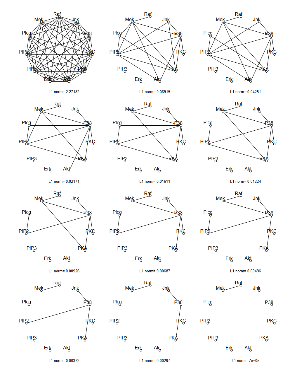
Example
Friedman and Hastie and Tibshirani "Sparse inverse covariance estimation with the graphical lasso", Biostatistics 2008
III. Regression for Networks
Neighborhood estimation problem
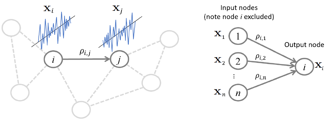
Regression problem for repating all other variables to a given variable
\begin{align} x_i = \sum_{k \neq i} \beta_{i,k} x_k + \epsilon_i, \end{align}Partial correlation, precision matrix, and regression coefficients
The partial correlation between a pair of variables, conditioned on all the rest, is related by a scalar to the $(i,j)$th element of the precision matrix.
A pair of variables $x_i$ and $x_j$ are conditionally independent if the linear regression coefficient $\beta_{i,j}=0$.
\begin{align} \rho_{i,j} = -\frac{\sigma^{i,j}}{\sqrt{\sigma^{i,i}\sigma^{j,j}}} &= -\beta_{i,j} \sqrt{\frac{\sigma^{i,i}}{\sigma^{j,j}}}, \end{align}Regression-based methods for estimating edges
Loop over all nodes and regress versus all others using your favorite regression method
can impose sparsity and other priors, can use efficient greedy methods
Linear Algebra view of Regression
The regression problem relating random variables $x_i$ is
\begin{align} x_i = \sum_{k \neq i} \beta_{i,k} x_k + \epsilon_i, \end{align}We use a vector of samples of each of the random variables $\{\mathbf x_1, ..., \mathbf x_m\}$
Then each neighborhood regression problem is
\begin{align} \mathbf x_i = \sum_{k \neq i} \mathbf x_k \beta_{i,k} + \boldsymbol\epsilon_i, \end{align}If we don't exclude the $i$th node from the sum (effectively allowing self-loops) we can write
\begin{align} \mathbf x_i = \mathbf X^T \boldsymbol\beta_{i} + \boldsymbol\epsilon_i, \end{align}Using matrix of data $\mathbf X$ where rows are samples $\mathbf x_i^T$ and columns are features. And $\boldsymbol\beta_{i}$ is the vector of coefficients $\beta_{i,k}$ relating the other nodes to the $i$th node.
Exercises
Draw a little network and relate it to $\mathbf X$ and $\boldsymbol\beta_{i}$
Combine all the regression problems for all nodes into a single equation
Least squares solution
Suppose our dataset matrix $\mathbf X$ is not invertible.
The least squares solution to $\mathbf X^T \mathbf B = \mathbf X^T$ is $\mathbf B = (\mathbf X^T)^\dagger \mathbf X^T$ using the pseudoinverse
If the SVD of $\mathbf X^T$ is $\mathbf U \mathbf S \mathbf V^T$ then we can write the SVD of $(\mathbf X^T)^\dagger$ as $\mathbf V \mathbf S\dagger \mathbf U^T$, where $S\dagger$ is a rectangular diagonal matrix with the inverses of the nonzero singular values of $\mathbf X^T$ on the diagonal (and zero otherwise).
Multiplying this out we get
\begin{align} \mathbf B &= (\mathbf X^T)^\dagger \mathbf X^T \\ &= (\mathbf V \mathbf S^\dagger \mathbf U^T)(\mathbf U \mathbf S \mathbf V^T) \\ &= \mathbf U_r \mathbf U_r^T \end{align}where $\mathbf U_r$ is the matrix of singular vectors for the $r$ nonzero singular values of $\mathbf X^T$.
Regression as Embedding
Consider the distances between rows of the matrix of regression coefficients $\mathbf B = \mathbf U_r \mathbf U_r^T $
\begin{align} d(i,j) &= \Vert \mathbf b^{(i)} - \mathbf b^{(j)} \Vert \\ &= \Vert \mathbf u_r^{(i)} \mathbf U_r^T - \mathbf u_r^{(j)} \mathbf U_r^T \Vert \\ &= \Vert (\mathbf u_r^{(i)} - \mathbf u_r^{(j)}) \mathbf U_r^T \Vert \\ &= \Vert \mathbf u_r^{(i)} - \mathbf u_r^{(j)} \Vert \\ \end{align}Where we use the fact that an orthogonal transformation does not change the distance (with a $\ell_2$-norm)
So the regression coefficient matrix is equivalent to a particular case of spectral embedding of the data
IV. Applications
Psychometric data
Estimating psychological networks and their accuracy: A tutorial paper S Epskamp, D Borsboom, EI Fried - Behavior Research Methods, 2018 - Springer
Software
Graph Visualization Software
NetworkX
igraph
- low-level (C++) implementation
- primarily R interface, less-functional python interface
- many more functions
import matplotlib.pyplot as plt
import networkx as nx
import numpy as np

A = np.random.rand(5,5)
A = A*(A>0.5)
G = nx.from_numpy_matrix(np.matrix(A), create_using=nx.DiGraph)
layout = nx.spring_layout(G)
nx.draw(G, layout)
#nx.draw_networkx_edge_labels(G, pos=layout)
nx.draw_networkx_labels(G, pos=layout)
plt.show();

Breast Cancer Data example
from sklearn import datasets
dat = datasets.load_breast_cancer()
Network based on Covariance of features
plt.imshow(C)
plt.colorbar();

Now visualize network
Covariance of Features for Malignant tumors
network0()

Covariance of Features for Benign tumors
network0()

Scikit-Learn GraphicalLasso()
import numpy as np
from sklearn.covariance import GraphicalLasso
Precision matrix of Features for Malignant tumors
network0()

Precision matrix of Features for Benign tumors
network0()

# author: Gael Varoquaux <gael.varoquaux@inria.fr>
# License: BSD 3 clause
# Copyright: INRIA

import numpy as np
from scipy import linalg
from sklearn.datasets import make_sparse_spd_matrix
from sklearn.covariance import GraphicalLassoCV, ledoit_wolf
import matplotlib.pyplot as plt

def rundemo():
    # #############################################################################
    # Generate the data
    n_samples = 60
    n_features = 20

    prng = np.random.RandomState(1)
    prec = make_sparse_spd_matrix(n_features, alpha=.98,
                              smallest_coef=.4,
                              largest_coef=.7,
                              random_state=prng)
    cov = linalg.inv(prec)
    d = np.sqrt(np.diag(cov))
    cov /= d
    cov /= d[:, np.newaxis]
    prec *= d
    prec *= d[:, np.newaxis]
    X = prng.multivariate_normal(np.zeros(n_features), cov, size=n_samples)
    X -= X.mean(axis=0)
    X /= X.std(axis=0)

    # #############################################################################
    # Estimate the covariance
    emp_cov = np.dot(X.T, X) / n_samples

    model = GraphicalLassoCV(cv=5)
    model.fit(X)
    cov_ = model.covariance_
    prec_ = model.precision_

    lw_cov_, _ = ledoit_wolf(X)
    lw_prec_ = linalg.inv(lw_cov_)

    # #############################################################################
    # Plot the results
    plt.figure(figsize=(10, 6))
    plt.subplots_adjust(left=0.02, right=0.98)

    # plot the covariances
    covs = [('Empirical', emp_cov), ('Ledoit-Wolf', lw_cov_),
            ('GraphicalLassoCV', cov_), ('True', cov)]
    vmax = cov_.max()
    for i, (name, this_cov) in enumerate(covs):
        plt.subplot(2, 4, i + 1)
        plt.imshow(this_cov, interpolation='nearest', vmin=-vmax, vmax=vmax,
               cmap=plt.cm.RdBu_r)
        plt.xticks(())
        plt.yticks(())
        plt.title('%s covariance' % name)


    # plot the precisions
    precs = [('Empirical', linalg.inv(emp_cov)), ('Ledoit-Wolf', lw_prec_),
             ('GraphicalLasso', prec_), ('True', prec)]
    vmax = .9 * prec_.max()
    for i, (name, this_prec) in enumerate(precs):
        ax = plt.subplot(2, 4, i + 5)
        plt.imshow(np.ma.masked_equal(this_prec, 0),
                   interpolation='nearest', vmin=-vmax, vmax=vmax,
                   cmap=plt.cm.RdBu_r)
        plt.xticks(())
        plt.yticks(())
        plt.title('%s precision' % name)
        if hasattr(ax, 'set_facecolor'):
            ax.set_facecolor('.7')
        else:
            ax.set_axis_bgcolor('.7')

    # plot the model selection metric
    plt.figure(figsize=(4, 3))
    plt.axes([.2, .15, .75, .7])
    plt.plot(model.cv_alphas_, np.mean(model.grid_scores_, axis=1), 'o-')
    plt.axvline(model.alpha_, color='.5')
    plt.title('Model selection')
    plt.ylabel('Cross-validation score')
    plt.xlabel('alpha')

    plt.show()
rundemo()


Sklearn Demo: Visualizing the stock market structure
Use is the daily variation in quote price to relate stocks: quotes that are linked tend to cofluctuate during a day.
Use sparse inverse covariance estimation to find which quotes are correlated conditionally on the others. Specifically, sparse inverse covariance gives us a graph, that is a list of connection. For each symbol, the symbols that it is connected too are those useful to explain its fluctuations.
# Author: Gael Varoquaux gael.varoquaux@normalesup.org
# License: BSD 3 clause

import sys

import numpy as np
import matplotlib.pyplot as plt
from matplotlib.collections import LineCollection

import pandas as pd

from sklearn import cluster, covariance, manifold

print(__doc__)


# #############################################################################
# Retrieve the data from Internet

# The data is from 2003 - 2008. This is reasonably calm: (not too long ago so
# that we get high-tech firms, and before the 2008 crash). This kind of
# historical data can be obtained for from APIs like the quandl.com and
# alphavantage.co ones.

symbol_dict = {
    'TOT': 'Total',
    'XOM': 'Exxon',
    'CVX': 'Chevron',
    'COP': 'ConocoPhillips',
    'VLO': 'Valero Energy',
    'MSFT': 'Microsoft',
    'IBM': 'IBM',
    'TWX': 'Time Warner',
    'CMCSA': 'Comcast',
    'CVC': 'Cablevision',
    'YHOO': 'Yahoo',
    'DELL': 'Dell',
    'HPQ': 'HP',
    'AMZN': 'Amazon',
    'TM': 'Toyota',
    'CAJ': 'Canon',
    'SNE': 'Sony',
    'F': 'Ford',
    'HMC': 'Honda',
    'NAV': 'Navistar',
    'NOC': 'Northrop Grumman',
    'BA': 'Boeing',
    'KO': 'Coca Cola',
    'MMM': '3M',
    'MCD': 'McDonald\'s',
    'PEP': 'Pepsi',
    'K': 'Kellogg',
    'UN': 'Unilever',
    'MAR': 'Marriott',
    'PG': 'Procter Gamble',
    'CL': 'Colgate-Palmolive',
    'GE': 'General Electrics',
    'WFC': 'Wells Fargo',
    'JPM': 'JPMorgan Chase',
    'AIG': 'AIG',
    'AXP': 'American express',
    'BAC': 'Bank of America',
    'GS': 'Goldman Sachs',
    'AAPL': 'Apple',
    'SAP': 'SAP',
    'CSCO': 'Cisco',
    'TXN': 'Texas Instruments',
    'XRX': 'Xerox',
    'WMT': 'Wal-Mart',
    'HD': 'Home Depot',
    'GSK': 'GlaxoSmithKline',
    'PFE': 'Pfizer',
    'SNY': 'Sanofi-Aventis',
    'NVS': 'Novartis',
    'KMB': 'Kimberly-Clark',
    'R': 'Ryder',
    'GD': 'General Dynamics',
    'RTN': 'Raytheon',
    'CVS': 'CVS',
    'CAT': 'Caterpillar',
    'DD': 'DuPont de Nemours'}


symbols, names = np.array(sorted(symbol_dict.items())).T

quotes = []

for symbol in symbols:
    print('Fetching quote history for %r' % symbol, file=sys.stderr)
    url = ('https://raw.githubusercontent.com/scikit-learn/examples-data/'
           'master/financial-data/{}.csv')
    quotes.append(pd.read_csv(url.format(symbol)))

close_prices = np.vstack([q['close'] for q in quotes])
open_prices = np.vstack([q['open'] for q in quotes])

# The daily variations of the quotes are what carry most information
variation = close_prices - open_prices


# #############################################################################
# Learn a graphical structure from the correlations
edge_model = covariance.GraphicalLassoCV(cv=5)

# standardize the time series: using correlations rather than covariance
# is more efficient for structure recovery
X = variation.copy().T
X /= X.std(axis=0)
edge_model.fit(X)

# #############################################################################
# Cluster using affinity propagation

_, labels = cluster.affinity_propagation(edge_model.covariance_)
n_labels = labels.max()

for i in range(n_labels + 1):
    print('Cluster %i: %s' % ((i + 1), ', '.join(names[labels == i])))

# #############################################################################
# Find a low-dimension embedding for visualization: find the best position of
# the nodes (the stocks) on a 2D plane

# We use a dense eigen_solver to achieve reproducibility (arpack is
# initiated with random vectors that we don't control). In addition, we
# use a large number of neighbors to capture the large-scale structure.
node_position_model = manifold.LocallyLinearEmbedding(
    n_components=2, eigen_solver='dense', n_neighbors=6)

embedding = node_position_model.fit_transform(X.T).T

# #############################################################################
# Visualization
plt.figure(1, facecolor='w', figsize=(10, 8))
plt.clf()
ax = plt.axes([0., 0., 1., 1.])
plt.axis('off')

# Display a graph of the partial correlations
partial_correlations = edge_model.precision_.copy()
d = 1 / np.sqrt(np.diag(partial_correlations))
partial_correlations *= d
partial_correlations *= d[:, np.newaxis]
non_zero = (np.abs(np.triu(partial_correlations, k=1)) > 0.02)

# Plot the nodes using the coordinates of our embedding
plt.scatter(embedding[0], embedding[1], s=100 * d ** 2, c=labels,
            cmap=plt.cm.nipy_spectral)

# Plot the edges
start_idx, end_idx = np.where(non_zero)
# a sequence of (*line0*, *line1*, *line2*), where::
#            linen = (x0, y0), (x1, y1), ... (xm, ym)
segments = [[embedding[:, start], embedding[:, stop]]
            for start, stop in zip(start_idx, end_idx)]
values = np.abs(partial_correlations[non_zero])
lc = LineCollection(segments,
                    zorder=0, cmap=plt.cm.hot_r,
                    norm=plt.Normalize(0, .7 * values.max()))
lc.set_array(values)
lc.set_linewidths(15 * values)
ax.add_collection(lc)

# Add a label to each node. The challenge here is that we want to
# position the labels to avoid overlap with other labels
for index, (name, label, (x, y)) in enumerate(
        zip(names, labels, embedding.T)):

    dx = x - embedding[0]
    dx[index] = 1
    dy = y - embedding[1]
    dy[index] = 1
    this_dx = dx[np.argmin(np.abs(dy))]
    this_dy = dy[np.argmin(np.abs(dx))]
    if this_dx > 0:
        horizontalalignment = 'left'
        x = x + .002
    else:
        horizontalalignment = 'right'
        x = x - .002
    if this_dy > 0:
        verticalalignment = 'bottom'
        y = y + .002
    else:
        verticalalignment = 'top'
        y = y - .002
    plt.text(x, y, name, size=10,
             horizontalalignment=horizontalalignment,
             verticalalignment=verticalalignment,
             bbox=dict(facecolor='w',
                       edgecolor=plt.cm.nipy_spectral(label / float(n_labels)),
                       alpha=.6))

plt.xlim(embedding[0].min() - .15 * embedding[0].ptp(),
         embedding[0].max() + .10 * embedding[0].ptp(),)
plt.ylim(embedding[1].min() - .03 * embedding[1].ptp(),
         embedding[1].max() + .03 * embedding[1].ptp())

plt.show()
