Dealing with Large Datasets
I.e. data is in external memory (e.g. hard drive(s)), a.k.a. out-of-core.
Also can be applied to data from network, sensor samples, etc.
- Incremental learning - algorithm consumes batch of data at a time rather than all of it
- Streaming - separate program loads data to feed into algorithm
- Reducing data - feature extraction/selection, hashing trick, dimensionality reduction, etc.
Approaches to parallelism
- JobLib
- Hashing trick
- scikit-learn Partial_fit()
- online learning
- streaming
numpy.linalg
- Use BLAS and LAPACK to provide efficient low level implementations of standard linear algebra algorithms.
- Those libraries may be provided by NumPy itself using C versions of a subset of their reference implementations
- but, when possible, highly optimized libraries that take advantage of specialized processor functionality are preferred.
- Examples of such libraries are OpenBLAS, MKL (TM), and ATLAS.
- Because those libraries are multithreaded and processor dependent, environmental variables and external packages such as threadpoolctl may be needed to control the number of threads or specify the processor architecture.
https://docs.scipy.org/doc/numpy/reference/routines.linalg.html
Linear algebra on several matrices at once
- As of version 1.8.0 several of the linear algebra routines are able to compute results for several matrices at once if they are stacked into the same array.
- indicated in the documentation via input parameter specifications such as a : (..., M, M) array_like.
- This means that if for instance given an input array a.shape == (N, M, M), it is interpreted as a “stack” of N matrices, each of size M-by-M.
- Similar specification applies to return values, for instance the determinant has det : (...) and will in this case return an array of shape det(a).shape == (N,).
- This generalizes to linear algebra operations on higher-dimensional arrays: the last 1 or 2 dimensions of a multidimensional array are interpreted as vectors or matrices, as appropriate for each operation.
Scikit-Learn
Popular Python ML toolbox, has several functions relevant to this course
- $\verb|sklearn.covariance|$: Covariance Estimators
- $\verb|sklearn.decomposition|$: Matrix Decomposition
- $\verb|sklearn.linear_model|$: Linear Models
- $\verb|klearn.manifold|$: Manifold Learning
- $\verb|sklearn.preprocessing|$: Preprocessing and Normalization
The Sklearn API
sklearn has an Object Oriented interface
Most models/transforms/objects in sklearn are Estimator objects
class Estimator(object):

    def fit(self, X, y=None):
        """Fit model to data X (and y)"""
        self.some_attribute = self.some_fitting_method(X, y)
        return self

    def predict(self, X_test):
        """Make prediction based on passed features"""
        pred = self.make_prediction(X_test)
        return pred

model = Estimator()
Unsupervised - Transformer interface
Some estimators in the library implement this.
Unsupervised in this case refers to any method that does not need labels, including unsupervised classifiers, preprocessing (like tf-idf), dimensionality reduction, etc.
The transformer interface usually defines two additional methods:
model.transform: Given an unsupervised model, transform the input into a new basis (or feature space). This accepts on argument (usually a feature matrix) and returns a matrix of the input transformed. Note: You need tofit()the model before you transform it.model.fit_transform: For some models you may not need tofit()andtransform()separately. In these cases it is more convenient to do both at the same time.
partial_fit()
- Replaces the fit() method
- applies to single instance or batch at a time
updates internal parameters
  est = SGDClassifier(...)
  est.partial_fit(X_train_1, y_train_1)
  est.partial_fit(X_train_2, y_train_2)
import numpy as np
from sklearn import linear_model

n_samples, n_features = 5000, 5

y = np.random.randn(n_samples)
X = np.random.randn(n_samples, n_features)

clf = linear_model.Ridge(alpha=0)

clf.fit(X, y)
print(clf.coef_,clf.intercept_)
X@clf.coef_ + clf.intercept_
y
clfi = linear_model.SGDRegressor(alpha=0)
for k in range(0,1000):
    k_rand = np.random.randint(0,len(X)-10)
    clfi.partial_fit(X[k_rand:k_rand+10,:], y[k_rand:k_rand+10]) # same as fit() for this case...
    if k%100==0:
        print(clfi.coef_,clfi.intercept_,np.linalg.norm(X@clf.coef_ + clf.intercept_ - y))
clfi = linear_model.SGDRegressor(alpha=0)
for k in range(0,10000):
    clfi.partial_fit(X, y) # same as fit() for this case...
    if k%1000==0:
        print(clfi.coef_,clfi.intercept_)
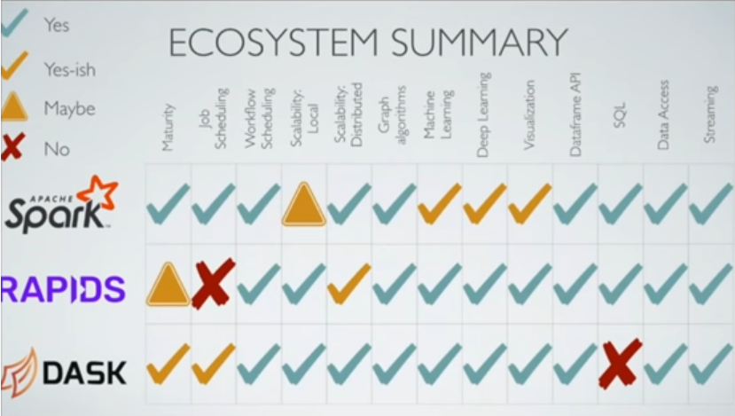
Is Spark Still Relevant: Spark vs Dask vs RAPIDS
https://www.youtube.com/watch?v=RRtqIagk93k
- Dask is functionally equivalent to Spark
- RAPIDS orders of magnitude faster than both because GPU's
- Spark = distributed dataframes on JVM on CPU
- Dask = distributed dataframes on CPU
- RAPIDS = distributed dataframes on GPU
- Why are enterprises still using spark?
- risk (spark is established, others brand new)
- support, consulting (only one: quansight), training
Ecosystem:
- Dask - Graph: networkX, ML: Dask-ml,scikit-learn,XGBoost, DL: TF,keras
- Spark - Graph: graphX, ML: MLlib,XGBoost, DL: ?
- RAPIDS: - Graph: cuGraph, ML: cuML, DL: Chainer, PyTorch,MXNet,DLPack
- Visualization with Dask: Datashader+Dask
- SQL: Dask has no SQL compiler, RAPIDS has blazingSQL, Spark has some
- Streaming: dask+streamz, RAPIDS custreamz, Spark streaming
Dask on Kubernetes
- Anaconda - Dask gateway
Pandas
pandas is a Python package providing fast, flexible, and expressive data structures designed to make working with “relational” or “labeled” data both easy and intuitive.
https://pandas.pydata.org/pandas-docs/stable/index.html
https://pandas.pydata.org/pandas-docs/stable/getting_started/10min.html
DataFrame
- a 2-dimensional labeled data structure with columns of potentially different types.
- can think of it like a spreadsheet or SQL table, or a dict of Series objects
- generally the most commonly used pandas object.
# https://pandas.pydata.org/pandas-docs/stable/getting_started/dsintro.html

import numpy as np
import pandas as pd

d = {'one': pd.Series([1., 2., 3.], index=['a', 'b', 'c']), 'two': pd.Series([1., 2., 3., 4.], index=['a', 'b', 'c', 'd'])}

df = pd.DataFrame(d)

print(df)
pd.DataFrame(d, index=['d', 'b', 'a'])
pd.DataFrame(d, index=['d', 'b', 'a'], columns=['two', 'three'])