Machine Learning

Keith Dillon
Fall 2018

Topic 3: Linear Algebra I

Outline

1. Vectors

2. Matrices

(in Python)

import numpy as np
from matplotlib import pyplot as plt
%matplotlib inline

Little code review workshop...

Let's convert last week's demo to C.

Linear Algebra

• Compact way to represent a tons of linear arithmetic. E.g. compute pairwise distances between a million points, solve huge linear system of equations, core steps in major algorithms.

• Very fast function libraries implementing these steps in low level languages. Freeing us to program in python, etc.

• Some key methods for regression, dimensionality reduction, classification.

• Jargon & notation used universally. Need to understand.

Goals: Learn to use a library of pre-optimized methods. Understand representation & application for Machine Learning.

Key Concepts

• Vectors

• Inner product - a.k.a. dot product

• Matrices - various representations

• Vector-matrix products - interpretation depends on representation

• Matrix-matrix product - transformations, or multiple vector-matrix products

• Eigendecomposition & Singular-Value Decomposition

Other Important Concepts

• Linear Systems

• Matrix inverse

• Matrix Identity

Part I. Vectors

Vectors

A $k$-dimensional vector $y$ is an ordered collection of $k$ real numbers $y_1 , y_2 , . . . , y_k$ and is written as $\textbf{y} = (y_1,y_2,...,y_k)$. The numbers $y_j$, for $j = 1,2,...,k$, are called the $\textbf{components}$ of the vector $y$. This is equivalent to a python-like 'list' vector, also called a row vector:

In math & physics, vectors more frequently written as column vectors:

$$\textbf{y} = \begin{bmatrix} y_1 \\y_2 \\ \vdots \\ y_k \end{bmatrix} = [y_1,y_2,...,y_k]^{T} $$

Swapping rows and columns = transposing. 1st column = top. 1st row = left.

Examples of vectors

A list of data for different "dimensions", for one person, product, etc.

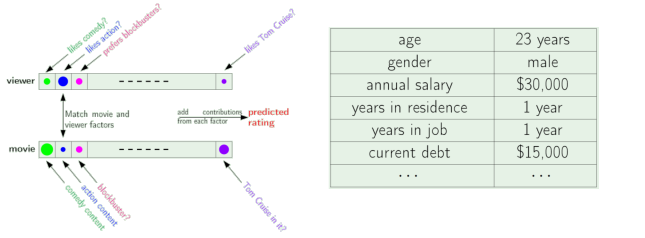
-Yaser Abu-Mostafa, Learning From Data

KEY FACT: The position in the vector is special, e.g. $x$ versus $y$.

NumPy Arrays for Vectors

x = np.array([2,0,1,8])

print(x)

Note Python is zero-based (like C & C++), but linear algebra writings are typically one-based.

x[0]

x[3]

Vector Statements

Let $\textbf{y}=(y_1,y_2,...,y_k)$ and $\textbf{z}=(z_1,z_2,...,z_k)$ be two k-dimensional vectors.

• $\textbf{y}=\textbf{z}$ when $y_j=z_j$ (j=1,2,...,k)

• $\textbf{y} \geq \textbf{z}$ or $\textbf{z} \leq \textbf{y}$ when $y_j \geq z_j$ (j=1,2,...,k)

• $\textbf{y}>\textbf{z}$ or $\textbf{z}<\textbf{y}$ when $y_j >z_j$ (j=1,2,...,k)

• $\textbf{0}$ is used to denote the null vector $(0, 0, ..., 0)$

E.g., $\textbf{x} \geq 0$, i.e., $\textbf{x} \geq \mathbf 0$, means $x_j \ge 0 $ for all $j$.

Scalar Multiplication

Scalar multiplication of a vector $\textbf{y} = (y_1, y_2, . . . , y_k)$ and a scalar α is defined to be a new vector $\textbf{z} = (z_1,z_2,...,z_k)$, written $\textbf{z} = \alpha\ \textbf{y}$ or $\textbf{z} = \textbf{y} \alpha$, whose components are given by $z_j = \alpha y_j$.

Vector addition

Addition of two k-dimensional vectors $\textbf{x} = (x_1, x_2, ... , x_k)$ and $\textbf{y} = (y_1,y_2,...,y_k)$ is defined as a new vector $\textbf{z} = (z_1,z_2,...,z_k)$, denoted $\textbf{z} = \textbf{x}+\textbf{y}$,with components given by $z_j = x_j+y_j$. (Subtraction is addition of a negative number of value.)

QUIZ:

Can you add: $ \begin{bmatrix} 3 \\ 1 \\ 5 \\ \end{bmatrix}$ and $\begin{bmatrix} 41 \\ 5 \\ 6 \\ 23 \\ \end{bmatrix}$? Why or why not?

Linear Combinations of Vectors

A linear combination of a collection of vectors $(\boldsymbol{x}_1, \boldsymbol{x}_2, \ldots, \boldsymbol{x}_m)$ is a vector of the form

$$a_1 \cdot \boldsymbol{x}_1 + a_2 \cdot \boldsymbol{x}_2 + \cdots + a_m \cdot \boldsymbol{x}_m$$

Just a combination of scalar multiplication and vector addition

Inner products

Three kinds of vector products, inner, outer, and cross products.

Most important is the dot or inner product, denoted as the multiplication of matching elements in one vector by the same element in the other vector, and summing these products.

If we have two vectors: ${\bf{x}} = (x_1, x_2, ... , x_k)$ and ${\bf{y}} = (y_1,y_2,...,y_k)$

The inner product is written: ${\bf{x}} \cdot {\bf{y}} = x_{1}y_{1}+x_{2}y_{2}+\cdots+x_{k}y_{k}$

If $\mathbf{x} \cdot \mathbf{y} = 0$ then $x$ and $y$ are orthogonal

What is $\mathbf{x} \cdot \mathbf{x}$?

If column vectors, ${\bf{x}} \cdot {\bf{y}} = \mathbf x^T \mathbf y$ (special case of Matrix-Matrix product)

We already saw a few inner products...

\begin{align} f(\mathbf x) = f(x_1, x_2, ..., x_n) = \text{sign}\left\{ \sum_{i=1}^{n}w_i x_i + b \right\} = \text{sign}(\mathbf w^T \mathbf x) \end{align}

Inner Product Geometrically

What does it tell you geometrically, i.e., what can it be used for?

Exercise

Make Jupyter notebook to demonstrate the operations in NumPy:

1. vector-scalar multiplication (just make up your own vectors and scalars)
2. vector-vector addition
3. dot products

Also test for yourself what happens when sizes do not match properly

Dot Product using NumPy

import numpy as np

w = np.array([1, 2])
v = np.array([3, 4])
np.dot(w,v)

11

w = np.array([0, 1])
v = np.array([1, 0])
np.dot(w,v)

0

w = np.array([1, 2])
v = np.array([-2, 1])
np.dot(w,v)

0

Part II. Matrices

Matrices

A matrix $M$ is a rectangular array of numbers, of size $m \times n$ as follows:

$M = \begin{bmatrix} x_{11} & x_{12} & x_{13} & \dots & x_{1n} \\ x_{21} & x_{22} & x_{23} & \dots & x_{2n} \\ \vdots & \vdots & \vdots & \ddots & \vdots \\ x_{m1} & x_{m2} & x_{m3} & \dots & x_{mn} \end{bmatrix}$

Where the numbers $x_{ij}$ are called the elements of the matrix. We describe matrices as wide if $n > m$ and tall if $n < m$. They are square iff $n = m$.

NOTE: naming convention for scalars vs. vectors vs. matrices.

Matrix Representations

Perhaps the main reason Linear Algebra can be so confusing is it is very abstract. This is because the matrix can describe many different things:

• Database table: rows are entries ("samples"), columns are features

• Coefficients in a linear system of equations

• Set of points. As columns (typical vector methods) or rows (typical statistics)

• Adjacency matrix describing graph

Can view all as a kind of table with different kinds of features & samples.

TIP: consider operations in terms of some representation you are comfortable with. E.g., inner products as customer & product profiles.

Exercise

Describe how you might convert these datasets into matrices:

1. Multiple bank customers from our earlier example

2. Multiple points in $(x,y,z)$.

3. DNA for many subjects.

If there's multiple options, note them all.

Modeling Networks with Matrices

A graph has nodes (e.g., states) and edges (e.g., transitions between states):

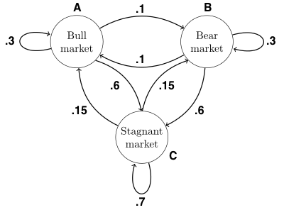
An adjacency matrix $\bf M$ compactly describes the graph, where the column index is initial state and row index is final state

$$\textbf{M} = \begin{bmatrix} 0.3 & 0.1 & 0.15\\ 0.1 & 0.3 & 0.15 \\ 0.6 & 0.6 & 0.7 \end{bmatrix} $$

Exercise

Write down the adjacency matrices for simple networks (from board)

Scalar Multiplication

Scalar multiplication of a matrix $\textit{A}$ and a scalar α is defined to be a new matrix $\textit{B}$, written $\textit{B} = \alpha\ \textit{A}$ or $\textit{B} = \textit{A} \alpha$, whose components are given by $b_{ij} = \alpha a_{ij}$.

Matrix Addition

Addition of two $m \times n$ -dimensional matrices $\textit{A}$ and $\textit{B}$ is defined as a new matrix $\textit{C}$, written $\textit{C} = \textit{A} + \textit{B}$, whose components $c_{ij}$ are given by addition of each component of the two matrices, $c_{ij} = a_{ij}+b_{ij}$.

Matrix Equality

Two matrices are equal when they share the same dimensions and all elements are equal. I.e.: $a_{ij}=b_{ij}$ for all $i \in I$ and $j \in J$.

Example:

$\textit{A} = \begin{bmatrix} 1 & 2 \\ 0 & 1 \\ \end{bmatrix}$

$\textit{B} = \begin{bmatrix} 2 & 0 \\ 1 & 4 \\ \end{bmatrix}$

$\textit{C} = \textit{A}+\textit{B} = \begin{bmatrix} 3 & 2 \\ 1 & 5 \\ \end{bmatrix}$

Matrix-Vector Multiplication

Two perspectives:

1. Linear combination of columns

2. Dot product of vector with rows of matrix

$\begin{bmatrix} 2 & -6 \\ -1 & 4\\ \end{bmatrix} \begin{bmatrix} 2 \\ -1 \\ \end{bmatrix} = ?$

Test both ways out.

Modeling State Transition with Matrix-vector Product

Recall we had the graph with adjacency matrix $\bf M$:

If the current state is described by vector $\mathbf s$, then the new state after one time-step is just the matrix-vector product $\mathbf M \mathbf s$.

$$\textbf{Ms} = \begin{bmatrix} 0.3 & 0.1 & 0.15\\ 0.1 & 0.3 & 0.15 \\ 0.6 & 0.6 & 0.7 \end{bmatrix} \begin{bmatrix} s_1\\ s_2 \\ s_3 \end{bmatrix} $$

Exercise

$$\textbf{M} = \begin{bmatrix} 0.3 & 0.1 & 0.15\\ 0.1 & 0.3 & 0.15 \\ 0.6 & 0.6 & 0.7 \end{bmatrix} $$

If the current state is described by vector $\mathbf s$, then the new state after one time-step is just the matrix-vector product $\mathbf M \mathbf s$.

Suppose $\mathbf s = \begin{bmatrix} 1 \\ 0 \\ 0 \end{bmatrix} $ ? How about $\mathbf s = \begin{bmatrix} 0.5 \\ 0.5 \\ 0 \end{bmatrix} $?

What do the results mean?

Matrix Multiplication

Multiplication of two two $m \times n$ -dimensional matrices $\textit{A}$ and $\textit{B}$ matrices is defined as a new matrix $\textit{C}$, written $\textit{C} = \textit{A}\textit{B}$, whose elements $c_{ij}$ are given by addition of each component of the two matrices, $c_{ij} = \sum_{k=1}a_{ik}b_{kj}$.

This can be memorized as row by column multiplication, where the value of each cell in the result is achieved by multiplying each element in a given row $i$ of the left matrix with its corresponding element in the column $j$ of the right matrix and adding the result of each operation together. This sum is the value of the new the new component $c_{ij}$.

We can take the product of matrices and vectors, under the assumption that the vector is oriented correctly and is of correct dimension (same rules as a matrix). In this case, we simply treat the vector as a $n \times 1$ or $1 \times n$ matrix.

(Note that $\textit{B}\textit{A} \neq \textit{A}\textit{B}$ in many cases.)

Example 1:

$\textit{A} = \begin{bmatrix} 1 & 2 \\ 0 & 1 \\ \end{bmatrix}$

$\textit{B} = \begin{bmatrix} 2 & 0 \\ 1 & 4 \\ \end{bmatrix}$

$\textit{C} = \textit{A}\textit{B} = \begin{bmatrix} 1 & 2 \\ 0 & 1 \\ \end{bmatrix} \begin{bmatrix} 2 & 0 \\ 1 & 4 \\ \end{bmatrix} = ?$

Example 1:

$\textit{C} = \textit{A}\textit{B} = \begin{bmatrix} 1 & 2 \\ 0 & 1 \\ \end{bmatrix} \begin{bmatrix} 2 & 0 \\ 1 & 4 \\ \end{bmatrix} = \begin{bmatrix} 4 & 8 \\ 1 & 4 \\ \end{bmatrix}$

Example 2:

$\begin{bmatrix} 1 & 2 \\ 0 & -3 \\ 3 & 1 \\ \end{bmatrix} \begin{bmatrix} 2 & 6 & -3 \\ 1 & 4 & 0 \\ \end{bmatrix} = ?$

Example 2:

$\begin{bmatrix} 1 & 2 \\ 0 & -3 \\ 3 & 1 \\ \end{bmatrix} \begin{bmatrix} 2 & 6 & -3 \\ 1 & 4 & 0 \\ \end{bmatrix} = \begin{bmatrix} 4 & 14 & -3\\ -3 & -12 & 0 \\ 7 & 22 & -9\\ \end{bmatrix}$

Example 3:

$\begin{bmatrix} 2 & 6 & -3 \\ 1 & 4 & 0 \\ \end{bmatrix} \begin{bmatrix} 1 & 2 \\ 0 & -3 \\ 3 & 1 \\ \end{bmatrix} = ?$

Example 3:

$\begin{bmatrix} 2 & 6 & -3 \\ 1 & 4 & 0 \\ \end{bmatrix} \begin{bmatrix} 1 & 2 \\ 0 & -3 \\ 3 & 1 \\ \end{bmatrix} = \begin{bmatrix} -7 & -17\\ 1 & -10 \\ \end{bmatrix}$

Example 4:

$\begin{bmatrix} 2 & -6 \\ -1 & 4\\ \end{bmatrix} \begin{bmatrix} 1 \\ 0 \\ \end{bmatrix} = ?$

Example 4:

$\begin{bmatrix} 2 & -6 \\ -1 & 4\\ \end{bmatrix} \begin{bmatrix} 1 \\ 0 \\ \end{bmatrix} = \begin{bmatrix} 2\\ -1\\ \end{bmatrix}$

QUIZ:

Can you take the product of $\begin{bmatrix} 2 & -6 \\ -1 & 4\\ \end{bmatrix}$ and $\begin{bmatrix} 12 & 46 \\ \end{bmatrix}$ ?

If question seems vague, list all possible ways to address this question.

Multiple State Transitions with Matrix-Matrix Products

Recall we had the graph with adjacency matrix $\bf M$:

If the current state is $\mathbf s$, the new state after one time-step is $\mathbf s' =\mathbf M \mathbf s$. Further, the new state after two time-steps is

$$\mathbf s'' = \textbf{Ms'} = \textbf{MMs} = \begin{bmatrix} 0.3 & 0.1 & 0.15\\ 0.1 & 0.3 & 0.15 \\ 0.6 & 0.6 & 0.7 \end{bmatrix} \begin{bmatrix} 0.3 & 0.1 & 0.15\\ 0.1 & 0.3 & 0.15 \\ 0.6 & 0.6 & 0.7 \end{bmatrix} \begin{bmatrix} s_1\\ s_2 \\ s_3 \end{bmatrix} $$

Multiple State Transitions with Matrix-Matrix Products

How do we represent three time-steps? ten?

Suppose the transition behavior of the graph changed over time, how would we represent that?

*** What could happen after infinite time steps?

(in practical world, that means just really many)

Matrix powers with NumPy

s = np.asarray([[.95],[.05],[.0]])
A = np.asarray([[.3,.1,.6],[.1,.3,.6],[.15,.15,.70]])

for i in [3, 5, 10, 50]:
    print('In ', i, 'years, we have:')
    print(np.linalg.matrix_power(A,i).dot(s))
    #print(np.dot(np.linalg.matrix_power(A,i),s)) # means comment

In  3 years, we have:
[[0.1706]
 [0.1634]
 [0.1665]]
In  5 years, we have:
[[0.166814]
 [0.166526]
 [0.166665]]
In  10 years, we have:
[[0.16666671]
 [0.16666662]
 [0.16666667]]
In  50 years, we have:
[[0.16666667]
 [0.16666667]
 [0.16666667]]

Matrix Transpose

The transpose of a matrix $\textit{A}$ is formed by interchanging the rows and columns of $\textit{A}$. That is

$a_{ij}^T = a_{ji}$

Example 1:

$\textit{A} = \begin{bmatrix} 1 & 2 \\ 0 & 1 \\ \end{bmatrix}$

$\textit{A}^{T} = ?$

Matrix Transpose

The transpose of a matrix $\textit{A}$ is formed by interchanging the rows and columns of $\textit{A}$. That is

$a_{ij}^T = a_{ji}$

Example 1:

$\textit{A} = \begin{bmatrix} 1 & 2 \\ 0 & 1 \\ \end{bmatrix}$

$\textit{A}^{T} = \begin{bmatrix} 1 & 0 \\ 2 & 1 \\ \end{bmatrix}$

Matrix Transpose

The transpose of a matrix $\textit{A}$ is formed by interchanging the rows and columns of $\textit{A}$. That is

$a_{ij}^T = a_{ji}$

Example 2:

$\textit{B} = \begin{bmatrix} 1 & 2 \\ 0 & -3 \\ 3 & 1 \\ \end{bmatrix}$

$\textit{B}^{T} = ?$

Matrix Transpose

The transpose of a matrix $\textit{A}$ is formed by interchanging the rows and columns of $\textit{A}$. That is

$a_{ij}^T = a_{ji}$

Example 2:

$\textit{B} = \begin{bmatrix} 1 & 2 \\ 0 & -3 \\ 3 & 1 \\ \end{bmatrix}$

$\textit{B}^{T} = \begin{bmatrix} 1 & 0 & 3 \\ 2 & -3 & 1 \\ \end{bmatrix}$

BONUS:

Show that $(\textit{A}\textit{B})^{T} = \textit{B}^{T}\textit{A}^{T}$.

Hint: the $ij$th element on both sides of the inequality is $\sum_{k}a_{jk}b_{ki}$

A Vector is just a Matrix with either $m=1$ or $n=1$

Recall matrices are $m \times n$ (note may use different letters).

A column vector is a matrix with $m$ rows and 1 column. Though we typically use different notation conventions for them versus "matrices" (what is it?)

$$ \boldsymbol{x} = \begin{bmatrix} x_{1}\\ x_{2}\\ \vdots\\ x_{m} \end{bmatrix} $$

A row vector is formed (and often written) as the transpose:

$$\boldsymbol{x}^T = [x_1, x_2, \ldots, x_n]$$

Vector Products as Matrix Products

If we have two vectors $\boldsymbol{x}$ and $\boldsymbol{y}$ of the same length $(n)$, then the dot product is give by matrix multiplication

$$\boldsymbol{x}^T \boldsymbol{y} = \begin{bmatrix} x_1& x_2 & \ldots & x_n \end{bmatrix} \begin{bmatrix} y_{1}\\ y_{2}\\ \vdots\\ y_{n} \end{bmatrix} = x_1y_1 + x_2y_2 + \cdots + x_ny_n$$

Wat happens if both are columns? Rows?

Differences between numpy vectors and arrays

• "Vector" implies a certain shape (either $m\times 1$ or $1\times n$ matrix, depending on field)
• "Array" implies just a list of numbers in computer memory, no special shape.

The distinction can be important. Ambiguities cause bugs. Data in various formats can be handled more efficienty by various algorithms.

• Numpy will let you get away with using arrays and will try to determine what you intended. Usually it will do what you intended...
• Tensorflow will not let you use arrays, but will demand that you specify two (or more) indices for vectors.
• SkLearn does not like matrices.

Exercises

1. Form two arrays or unoriented vectors. These are numpy arrays whose shape is something like (n,). Take their dot product.
2. Form two vectors or oriented vectors. These will have shapes like (n,1) or (1,n). Take their dot product. If you used the same numeric values in as in 1, the answers will be the same.
3. Reverse the order of the multiplication in 2 (reverse the order of the arguments in the dot() function). Are the two vectors still conformable? What shape do you expect the answer to have? What shape does it have?
4. Generate the same result as in 3, using unoriended vectors (arrays).

NumPy vectors can be formed/defined various ways, as simple array versus matrix. Functions will typically guess what you mean.

x = np.array([1,2,3,4])
print(x)
print(x.shape)
x = x.reshape(4,1)
print(x)
print(x.shape)

[1 2 3 4]
(4,)
[[1]
 [2]
 [3]
 [4]]
(4, 1)

x_T = x.transpose()
print (x_T)
print (x_T.shape)
print(x.T)

[[1 2 3 4]]
(1, 4)
[[1 2 3 4]]