Outline
Advanced matrix methods
Eigen-stuff
Eigendecomposition-based methods: SVD, PCA, LDA
import numpy as np
from matplotlib import pyplot as plt
%matplotlib inline
Part III. Advanced Matrix Methods
Properties of Matrices
For three matrices ${A}$, ${B}$, and ${C}$ we have the following properties
Commutative Law of Addition: ${A} + {B} = {B} + {A}$
Associative Law of Addition: $(\textit{A} + \textit{B}) + \textit{C} = \textit{A} + (\textit{B} + \textit{C})$
Associative Law of Multiplication: $\textit{A}(\textit{B}\textit{C}) = (\textit{A}\textit{B})\textit{C}$
Distributive Law: $\textit{A}(\textit{B} + \textit{C}) = \textit{A}\textit{B} + \textit{A}\textit{C}$
Identity: There is the matrix equivalent of one. We define a matrix ${I_n}$ of dimension $n \times n$ such that the elements of ${I_n}$ are all zero, except the diagonal elements $i=j$; where $i_{ii} = 1$
Zero: We define a matrix 0 of $m \times n$ dimension as the matrix where all components $ij$ are 0
Identity Matrix
$I_3 = \begin{bmatrix} 1 & 0 & 0\\ 0 & 1 & 0 \\ 0 & 0 & 1\\ \end{bmatrix}$
Here we can write $\textit{I}\textit{B} = \textit{B}\textit{I} = \textit{B}$ or $\textit{I}\textit{I} = \textit{I}$
Again, it is important to reiterate that matrices are not in general commutative with respect to multiplication. That is to say that the left and right products of matrices are, in general different.
$AB \neq BA$
import numpy as np
np.eye(3)
Exercise
Use your Jupyter notebook to demonstrate the following operations using NumPy:
- matrix-vector multiplication
- matrix-matrix ultiplication
- the six matrix properties
Also test for yourself what happens when sizes do not match properly
NumPy Example 1:
A = np.asarray([[1,2],[4,5]])
B = np.asarray([[3,4,6],[4,5,7],[7,8,9]])

#A + B
np.matmul(A,B)
NumPy Example 2:
A = np.asarray([[1,2],[4,5],[1,2]])
B = np.asarray([[3,4],[5,7],[7,8]])
B = B.transpose()

#A + B
#print(np.matmul(A,B))
print(A@B)
A = np.asarray([[1,2],[4,5],[1,2]])
B = np.asarray([[3,4],[5,7],[7,8]])

# np.matmul(A,B.transpose())
A@B.transpose()
Linear System of Equations
A system of equations of the form: \begin{align*} a_{11}x_1 + \cdots + a_{1n}x_n &= b_1 \\ \vdots \hspace{1in} \vdots \\ a_{m1}x_1 + \cdots + a_{mn}x_n &= b_m \end{align*} can be written as a matrix equation: $$ A\mathbf{x} = \mathbf{b} $$
Can describe problems in Physics, Engineering, Regression, etc.
In Linear Algebra, can be directly solved as $$ \mathbf{x} = A^{-1}\mathbf{b} $$
The inverse generally doesn't exist unless conditions are just right. Know them?
Inverse of a Matrix
The inverse of a square $n \times n$ matrix $X$ is an $n \times n$ matrix $X^{-1}$ such that
$$X^{-1}X = XX^{-1} = I$$
Where $I$ is the identity matrix, an $n \times n$ diagonal matrix with 1's along the diagonal.
If such a matrix exists, then $X$ is said to be invertible or nonsingular, otherwise $X$ is said to be noninvertible or singular.
NumPy Inverse
A = np.asarray([[1,2],[4,5]])

iA = np.linalg.inv(A)

print(A@iA)
print(np.matmul(A,iA))
A = np.random.randint(0, 10, size=(3, 3))
A_inv = np.linalg.inv(A)
print(A)
print(A_inv)
print(np.matmul(A,A_inv))
IMPORTANT NOTE: "hard zeros" rarely exist in real world due to limited numerical precision.
Believe it or Not
You know how to solve linear systems (solve one equation for one variable, plug into next equation, ...)
The inverse programmatically accomplishes the same steps!
In the real world you will very rarely compute an inverse. Not even to solve a system with an invertible matrix. Mainly just used as sub-steps inside other algorithms you use.
Part IV. Eigendecompositions and Applications
Eigenvalues and Eigenvectors
Let $\bf A$ be a given nonzero square matrix of dimension $n \times n$. Consider the following equation:
$${\bf A}{\bf x} = \lambda {\bf x}$$
This equation is called an eigenvalue equation. Here $\bf A$ is a given square matrix, $\bf x$ is an unknown vector, and $\lambda$ is an unknown scalar. The problem of finding $\lambda$'s and nonzero ${\bf x}$'s that satisfy the eigenvalue equation is called the eigenvalue problem.
Super-important Question: what would this mean for a state-transition (suppose initial state is engevector $\mathbf x$)?
Eigenvalue and Eigenvectors: Network intuition
Eigenvectors are those states which remain unchanged over time (except for overall scaling, perhaps).
Eigenvalues are the amount of scaling over time: decay, explode, or stay-constant.
Can you guess how we might compute eigenvectors (at least one)?
Eigenvector of the Internet
PageRank algorithm computes eigenvector of largest eigenvalue of internet network.
Power method used to compute the eigevector from the huge adjacency matrix
"The Mathematics Behind Google"
Eigenvalue Decomposition
Let $\bf A$ be a given nonzero square matrix of dimension $n \times n$. The eigenvalue equation is:
$${\bf A}{\bf x} = \lambda {\bf x}$$
This will have at most $n$ solutions (e.g., ${\bf A}{\bf x}_i = \lambda_i {\bf x}_i$). If our matrix has $n$ eigenvalues, we can combine the equations for them and form the matrix decomposition:
$${\bf A}{\bf X} = {\bf X} \Lambda$$
$\mathbf X$ is a matrix with eigenvectors as columns, and $\Lambda$ is a diagonal matrix with eigenvalues along the diagonal (typically ordered by size).
Write out a simple example and check!
Orthogonal Components
...depending on class background...
Breaking up vector
Bases
Orthonormal matrices
what a matrix-vector product does (in terms of eigenvalues)
Eigenvalue Decomposition
$${\bf A}{\bf x} = \lambda {\bf x} \leftarrow \text{know this}$$
$${\bf A}{\bf X} = {\bf X} \Lambda$$
One more trick, and eigenvector matrix $\mathbf X$ is special in that $\mathbf X^T = \mathbf X^{-1}$, (known as an orthonormal matrix), so we can write the decomposition as:
$${\bf A} = {\bf X} \Lambda {\bf X^T} \leftarrow \text{know this}$$
Rank, Nullspace, Rowspace, and all that
...depending on class background...
Consider the product $\mathbf A \mathbf v = {\bf X} \Lambda {\bf X^T} \mathbf v$ when some eigenvalues are zero.
Eigendecomposition-Related Methods
There are many methods based on the idea of eigenvectors as a fundamental component of the data in the matrix (with the corresponding eigenvalue giving the importance of that component).
Here's some very common ones you might come across. They only take a few lines of code plus eig() or svd().
Singular Value Decomposition (SVD) - essentially an Eigenvalue decomposition of the "matrix squared" ($\mathbf A \rightarrow \mathbf A^T \mathbf A$ and $\mathbf A \mathbf A^T$). More broadly usable.
Principal Component Analysis (PCA) - Dim. reduction method. Essentially just SVD of matrix after some optional preprocessing (e.g., normalize).
...continued
Eigendecomposition-Related Methods (continued)
Linear Discriminant Analysis (LDA) - Classification method. Given multiple data matrices (one per class), computes eigenvectors which best discriminate between the classes.
Cannonical Component Analysis (CCA) - Feature extraction method. Given two data matrices (describing different things), find eigenvector which gives related component in both matrices.
Spectral Graph Theory - field that analyzes eigendecomposition of graph adjacency (and related) matrices. Methods for graph embedding and partitioning.
Eigenvalue Decomposition in NumPy
s = np.asarray([[.95],[.05],[.0]])
A = np.asarray([[.3,.1,.6],[.1,.3,.6],[.15,.15,.70]])

np.linalg.matrix_power(A,20).dot(s)
np.linalg.eig(A)
Exercises
Make a little matrix and compute its decompositions. Anyone find interesting ones?
Multiply the parts back together and reconstruct the original matrix
Eigenvalue Decomposition Details
- Matrix must be square
- If matrix not symmetric, may need "generalized eigenvalues", complex numbers
What does a symmetric vs. asymmetric adjacency imply about the graph?
What might a lack of nice (real scalar) eigevalues say about matrix powers?
Singular-Value Decomposition (SVD)
A related decomposition that works for asymmetric & rectangular matrices.
Core step in Principal Component Analysis, a (super) widely-used method for dimensionality reduction.
Also used in recommendation systems to factor matrices describing user preferences.
Many other applications.
Eigenvector decompotisiton: ${\bf A} = {\bf X} \boldsymbol\Lambda {\bf X^T}$
Singular-value decomposition: ${\bf A} = {\bf U} {\bf S} {\bf V^T}$
Singular-Value Decomposition (SVD)
Eigenvector decompotisiton: ${\bf A} = {\bf X} \boldsymbol\Lambda {\bf X^T}$
Singular-value decomposition: ${\bf A} = {\bf U} {\bf S} {\bf V^T}$
- $\bf U$ has "left singular vectors" as columns.
- $\bf V$ has "right singular vectors" as columns.
- $\bf S$ is a rectangular diagonal matrix with singularvalues along the diagonal (ordered by size).
Rowspace, Nullspace and Rank
...depending on class background...
Consider that matrix-vector product again.
Exercises
Compute the eigenvalue decomposition and SVD of a matrix and looks for similarities.
Reconstruct the matrix from its SVD.
BONUS: figure out how to compute the SVD from eig
SVD for Dimensionality Reduction
https://en.wikipedia.org/wiki/Principal_component_analysis
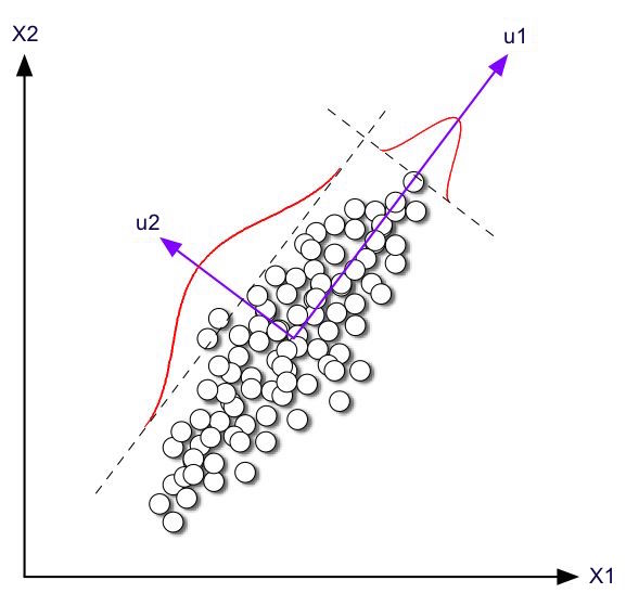
- View matrix as a collection of points in space...
- Large singular values tell directions (singular vectors) of high variation
- Small singular values tell directions of small variation.
PCA essentially keeps largest singular values and their singular vectors.
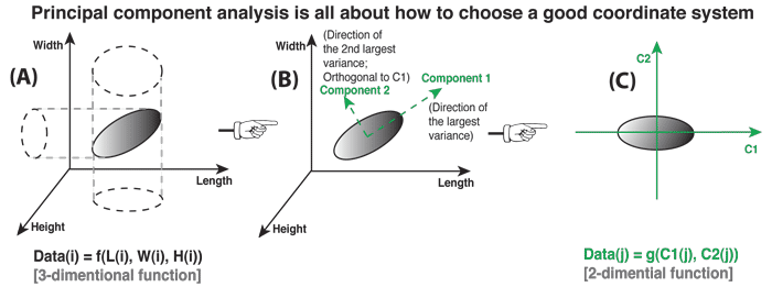
Principal Component Analysis (PCA)
In a nutshell, this is what PCA is all about: Finding the directions of maximum variance in high-dimensional data and project it onto a smaller dimensional subspace while retaining most of the information.
Lab
Load IRIS dataset and plot as points in space (choose a couple features)
Compute SVD and plot largest singular vectors.
What happens if data is far from origin? How can we fix that?
Now how do we look at the data in the "principal directions"?
Questions
How do we pick the directions of largest variation?
How do we decide how many to use?
How decide which directions variation to ignore/discard?
Linear Discriminant Analysis (LDA)
Recall PCA uses singular vectors to give directions of largest data variation.
LDA uses singular vectors to give direction of largest difference between two classes.
Algorithm is very simple. But we can just stick to SkLearn.
from sklearn.discriminant_analysis import LinearDiscriminantAnalysis
Lab
# load IRIS dataset

# make data matrix X and labels y

# Create an instance of the class
lda = LinearDiscriminantAnalysis(n_components = 2)

# Fit the model to the data
#lda.fit(X,y)

# Plot data on discriminants

# Classify data...