Outline
Average distances between points in high-dimensional space
Volumes in high-dimensional space
Feature Engineering
import numpy as np
from matplotlib import pyplot as plt
%matplotlib inline
Problems with some methods for large datasets
Efficiency: What is order of computation?
Curse of dimensionality: need exponentially more data for more dimensions
Consider how the combo of #1 and #2 compounds difficulties
For which methods might this be a problem?
The Curse of Dimensionality
Problems that arise in "high" dimensions "$d>3$" (i.e. most datasets):
- Nearest points are often extremely far away, so that differences between the distances tend to be relatively smaller.
- Computational cost of managing long data vectors increases.
- Sampling becomes inefficient as the number of data points required to adequately describe the sample space increases exponentially!
Simulation: Average Distances between Random Points
Generate a uniformly-distributed (equal probability of being at each point) set of points in a $d$-dimensional unit hypercube (side = 1 unit). 3D shown below:
Compute average distances between all pairs and see what happens...
NumPy Loop
N_x = 100; # number of points to use
N_d = 30;  # max number of dimensions to test

avg_dist = np.zeros(N_d);

for d in np.arange(1,N_d): # loop over dimensions
    X = np.random.rand(N_x,d); # make d-dimensional uniform random data
    for i in np.arange(0,N_x): # now loop over pairs of points
        x_i = X[i]
        for j in np.arange(0,N_x):
            x_j = X[j]
            if i != j:
              #print(i,j,d,x_i,x_j,np.linalg.norm(x_i-x_j))
              avg_dist[d] = avg_dist[d] + np.linalg.norm(x_i-x_j)/N_x/(N_x-1.)
Average Distance Between Pairs
plt.plot(np.arange(1,N_d),avg_dist[1:]);
#plt.plot(np.arange(1,N_d),np.sqrt(np.arange(1,N_d)));

plt.ylabel('Distance');
plt.xlabel('Dimensions d');
#plt.legend(['Average Dist','sqrt(d)']);

Exercises
Calculate max possible distance in hyper cube in 1, 2, and 3 dimensions.
Calculate amount of volume within 10 percent of edge in 1, 2, and 3 dimensions (square or circle).
What's going on? Consider Volume in Hyperspace
Consider a square with sides of length $l$. We wish to compute the fraction of total volume occupied by a small margin as shown in the following figure (the gray part):
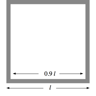
In 2D: $V_M = l^2 - (0.9 l)^2 = l^2 (1 - 0.9^2) = 0.19 \times l^2$
In 3D: $V_M = l^3 - (0.9 l)^3 = l^3 (1 - 0.9^3)= 0.27 \times l^3$
In 50D: $V_M = l^{50} - (0.9 l)^{50} = l^{50} (1 - 0.9^{50})= 0.9948 \times l^{50}$
In $d$-D for large $d$: $V_M \approx l^d$ i.e. space is almost all margin
Analysis of the effect of Dimensionality on Marginal Volume of a Hypercube
def hyperMarginRatio(d = 1, marginRatio = .1, edgeLen = 1):
    TotVolume = edgeLen**d

    HoleLen = edgeLen*(1-marginRatio)
    HoleVolume = HoleLen**d

    marginRatio = (TotVolume - HoleVolume)/TotVolume

    print ("When dimension = " + str(d) + " and the margins are " + str(marginRatio*100) + "% of the total edge length:")
    print ("   Total volume = " + str(TotVolume))
    print ("   Hole volume = " + str(HoleVolume))
    print ("   So as a ratio,")
    print (str(100*marginRatio) + "% of the volume is in the margins.")
    print ("")
    return marginRatio
d2 = hyperMarginRatio(d = 2)
maxD = 50
marginRatio = .05


marginRatios = []
X = range(1,maxD+1, 10)

for d in X:
    appenders = round(hyperMarginRatio(d, marginRatio = marginRatio), 2)
    marginRatios.append(appenders)
Margins volume versus Dimension
%matplotlib inline
import matplotlib.pyplot as plt
plt.plot(X, marginRatios)
plt.title('Ratio of margins volume as a function of dimension');

The effect of Dimensionality on Required Sampling Density
Another perspective: as dimension increases, points become sparsely distributed
Consider a $d$-dimensional grid to sample uniformly $N_s^d$ grid points needed.
The density of points in a fraction of the volume: $N_{total} r^d$
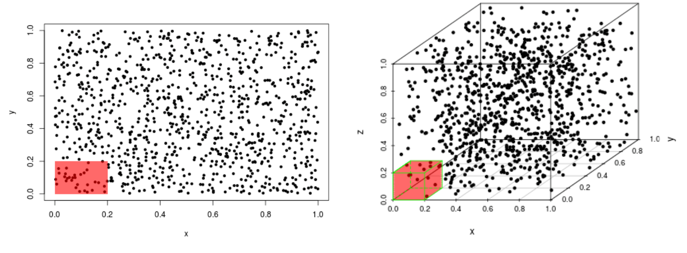
Simulation
$1000$ randomly generated, count points which land in $20\%$ of the range of each feature.
The rectangle in $2d$ captures $3.1\%$ of the data points
The cube in $3d$ captures only $0.5\%$ of total data points.
Conclusion
So what does this mean?
to ability to use data to describe space for a classifier
to ability to test methods with randomly-simulated samples
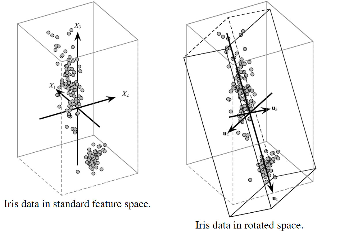
Addressing the Curse of Dimensionality: Feature Engineering
Need to lower the dimensionality of the metric space ($S$) in $\mathbb{R}^n$ while maintaining the ordering within the metric space.
If we have a set of points $\bf{x} \in X$ in we need to find corresponding set of points $\bf{u}$ in a new metric space $U$ over the field $\mathbb{R}^m$, such that $m < n$ and the metric space is almost preserved by some finite margin of error:
$$\|x_{i}-x_{j}\|_2 \leq \|u_{i}-u_{j}\|_2 \leq (1+\epsilon)\|x_{i}-x_{j}\|_2$$
Feature Engineering
This process, applied professionally, is called Feature engineering
Half of Machine Learning class and half the work you will do in practice.
Largely a guess-and-check process of attempting to generate the mapping to the new metric space through methods meant to model the underlying meaning, thus making the mapping S→US→U.
Oftentimes the quality of the feature engineering is only known after the fact.
Feature Engineering Examples
Discard variables (i.e. dimensions) for which the information is minimal
Replace multiple related variables with their sum or average.
Replace multiple related variables with a smaller set of more general combinations
Dimensionality Reduction via PCA