Outline
Features
Distances & Norms
Overfitting
Performance metrics
import numpy as np
from matplotlib import pyplot as plt
%matplotlib inline
Formal Classification Problem
Mathematically, a classifier is a function or model $f$ that predicts the class label for a given input example ${\mathbf x}$, that is
$$\hat{y} = f({\bf x})$$
The value $\hat{y}$ belongs to a set $\{c_1,c_2,...,c_k\}$, each $c_i$ is a class label.
To build the model we use training set, a set of points with known class labels.
Once the model $f$ is known, we can automatically predict the class for any new data point.
Formal Classification Problem
Mathematically, a classifier is a function or model $f$ that predicts the class label for a given input example ${\bf x}$, that is
$$\hat{y} = f({\bf x})$$
- The value $\hat{y}$ belongs to a set $\{c_1,c_2,...,c_k\}$, each $c_i$ is a class label.
The quality of the model is inherently determined by the quality and accuracy of the training set, an important consideration upon evaluating any implementation of a model.
Several standardized data sets that have been tested and evaluated over many years.
Scikits has a very good sample of the standardized data sets set up to be easily accessed from the standard api, as discussed here.
The Simplest Function Imaginable
- Using a training set with samples $\mathbf x_i$ and known labels $y_i$
- How use that to decide new label $y'$ for new sample $\mathbf x'$?
The Simplest Function Imaginable
- Using a training set with samples $\mathbf x_i$ and known labels $y_i$
- How use that to decide new label $y'$ for new sample $\mathbf x'$?
- First Idea: Lookup table, a stored table of input-output pairs
- E.g., Tables of triginometric and other functions in books or ROM
- Lists of patient symptoms and disease they had
PROBLEMS:
- What if there's no perfect match?
- How do we (and they) handle continuous real values?
- What if identical-looking patients have different diseases?
Fisher's Iris Data Set
Extract below of the standardized Fisher's Iris dataset, originally collected and categorized by hand; the complete data forms a $150\times 4$ data matrix.
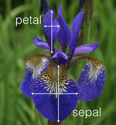
The set gives the sepal length, sepal width, petal length, and petal width in centimeters, and the type or class of the Iris flower, for 150 flowers.
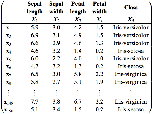
What are the samples? features?
Iris Classification Problem
The flowers in the Fisher dataset were classified by experts. Or goal (as non-experts) is to use this info to learn how to predict the class of a new flower, given the same four length & width measurements (but not the class).
How does this fit into the formal classification problem?
How might we do that? (besides hiring the experts). E.g. $\mathbf x' = \begin{pmatrix}6, 3, 4, 2\end{pmatrix}$, Class=?
The "1-Nearest-Neighbor" Algorithm
Starting with training set of samples with known labels.
Given sample with unknown label, assign label of closest sample from training set.
Distance = $d\left(\text{"training_sample"}, \text{"test_sample"}\right)$
But how do we determine closest training sample?
Exercise
Load IRIS dataset & implement a 1-$NN$ algorithm to classify new vectors.
from sklearn import datasets
iris = datasets.load_iris()

dir(iris)
(iris.data, iris.target)
iris.data[52]
Distance Metrics
Ex: Euclidean distance between two vectors $a$ and $b$ in $\mathbb{R}^{n}$:
$$d(\mathbf a,\mathbf b) = \sqrt{\sum_{i=1}^{n}(b_i-a_i)^2}$$
But this may not make sense for flower dimensions. Many alternatives...
A metric $d(\mathbf x,\mathbf y)$ must satisfy four particular conditions to be considered a metric:
- Non-negativity: $d(\mathbf x,\mathbf y) \geq 0$
- Zero upon equality: $d(\mathbf x,\mathbf y) = 0 \iff \mathbf x = \mathbf y$
- Commutativity of arguments: $d(\mathbf x,\mathbf y) = d(\mathbf y,\mathbf x)$
- Triangle Inequality: $d(\mathbf x,\mathbf z) \leq d(\mathbf x,\mathbf y) + d(\mathbf y,\mathbf z)$
Manhattan or "Taxicab" Distance, also "Rectilinear distance"
Measures the relationships between points at right angles, meaning that we sum the absolute value of the difference in vector coordinates.
This metric is sensitive to rotation.
$$d_{M}(a,b) = \sum_{i=1}^{n}|(b_i-a_i)|$$
Exercise
Does it fulfill the 4 conditions?
Try using the above distance metrics to compare flowers. Which makes most sense?
Manhattan or "Taxicab" Distance, also "Rectilinear distance"
Measures the relationships between points at right angles, meaning that we sum the absolute value of the difference in vector coordinates.
This metric is sensitive to rotation.
$$d_{M}(a,b) = \sum_{i=1}^{n}|(b_i-a_i)|$$
- Non-negativity: $d(\mathbf x,\mathbf y) \geq 0$
- Zero upon equality: $d(\mathbf x,\mathbf y) = 0 \iff \mathbf x = \mathbf y$
- Commutativity of arguments: $d(\mathbf x,\mathbf y) = d(\mathbf y,\mathbf x)$
- Triangle Inequality: $d(\mathbf x,\mathbf z) \leq d(\mathbf x,\mathbf y) + d(\mathbf y,\mathbf z)$
Chebyschev Distance
The Chebyschev distance or sometimes the $L^{\infty}$ metric, between two vectors is simply the the greatest of their differences along any coordinate dimension:
$$d_{\infty}(\mathbf a,\mathbf b) = \max_{i}{|(b_i-a_i)|}$$
Chebyschev Distance
The Chebyschev distance or sometimes the $L^{\infty}$ metric, between two vectors is simply the the greatest of their differences along any coordinate dimension:
$$d_{\infty}(\mathbf a,\mathbf b) = \max_{i}{|(b_i-a_i)|}$$
- Non-negativity: $d(\mathbf x,\mathbf y) \geq 0$
- Zero upon equality: $d(\mathbf x,\mathbf y) = 0 \iff \mathbf x = \mathbf y$
- Commutativity of arguments: $d(\mathbf x,\mathbf y) = d(\mathbf y,\mathbf x)$
- Triangle Inequality: $d(\mathbf x,\mathbf z) \leq d(\mathbf x,\mathbf y) + d(\mathbf y,\mathbf z)$
Cosine Distance
The cosine distance between two vectors is a measure of rotational relationship rather than magnitude. It is frequently used in bioinformatics where total magnitude changes little as there are often hundreds if not thousands of "coordinates", but relationships among coordinate dimensions may change dramatically.
$$d_{Cos}(\mathbf a,\mathbf b) = \frac{\mathbf a \cdot \mathbf b}{\|\mathbf a\|\|\mathbf b\|}$$
Note: actually helps some with the curse of dimensionality (covered later), as it discards some info... reducing dimensionality.
Cosine Distance
The cosine distance between two vectors is a measure of rotational relationship rather than magnitude. It is frequently used in bioinformatics where total magnitude changes little as there are often hundreds if not thousands of "coordinates", but relationships among coordinate dimensions may change dramatically.
$$d_{Cos}(\mathbf a,\mathbf b) = 1-\frac{\mathbf a \cdot \mathbf b}{\|\mathbf a\|\|\mathbf b\|}$$
Note: actually helps some with the curse of dimensionality (covered later), as it discards some info... reducing dimensionality.
- Non-negativity: $d(\mathbf x,\mathbf y) \geq 0$
- Zero upon equality: $d(\mathbf x,\mathbf y) = 0 \iff \mathbf x = \mathbf y$
- Commutativity of arguments: $d(\mathbf x,\mathbf y) = d(\mathbf y,\mathbf x)$
- Triangle Inequality: $d(\mathbf x,\mathbf z) \leq d(\mathbf x,\mathbf y) + d(\mathbf y,\mathbf z)$
Exercise
Implement the metrics in numpy manually and compute distances between:
$ \begin{bmatrix} 1 \\ 2 \\ 3 \\ 4 \end{bmatrix}$ and $ \begin{bmatrix} 5 \\ 6 \\ 7 \\ 8 \end{bmatrix}$
import numpy as np
import scipy
x = np.array([1,2,3,4])
y = np.array([5,6,7,8])
print(1-np.dot(x,y)/(np.linalg.norm(x)*np.linalg.norm(y)))

print(scipy.spatial.distance.cosine(x,y))

dir(scipy.spatial.distance)
Exercise
Try using the above distance metrics to compare flowers. Which makes most sense?
Hamming or "Rook" Distance
The hamming distance can be used to compare nearly anything to anything else. It is used in comparison of strings of equal length, and defined as the number of differences in characters between two strings, ie:
$$d_{hamming}('bear', 'beat') = 1$$ $$d_{hamming}('cat', 'cog') = 2$$ $$d_{hamming}('01101010', '01011011') = 3$$
Edit distance
Similar to hamming distance, but also includes insertions and deletions, and so can compare strings of any length to each other.
$$d_{edit}('lead', 'gold') = 4$$ $$d_{edit}('monkey', 'monk') = 2$$ $$d_{edit}('lucas', 'mallori') = 8$$
Norms
A norm is a vector "length", essentially a distance for a single vector (i.e., distance from origin $d(\mathbf x,0)$. Often denoted as $\Vert \mathbf x \Vert$.
Similar properties required.
- Non-negativity: $\Vert \mathbf x \Vert \geq 0$
- Zero upon equality: $\Vert \mathbf x \Vert = 0 \iff \mathbf x = \mathbf y$
- Absolute scalability: $\Vert \alpha \mathbf x \Vert = |\alpha| \Vert \mathbf x \Vert$ for scalar $\alpha$
- Triangle Inequality: $\Vert \mathbf x + \mathbf z\Vert \leq \Vert \mathbf x\Vert + \Vert \mathbf z\Vert$
What are the norm versions of our distances?
Norms and Lebesgue space
The $L^{p}$, or Lebesgue space, consists of all of functions of the form:
$\|f\|_{p} = (|x_{1}|^{p}+|x_{2}|^{p}+|x_{n}|^{p}+)^{1/p}$
This mathematical object is known as a p-norm.
$p$-norm: For any $n$-dimensional real or complex vector. i.e. $x \in \mathbb{R}^n \text{ or } \mathbb{C}^n$
$$ \|x\|_p = \left(|x_1|^p+|x_2|^p+\dotsb+|x_n|^p\right)^{\frac{1}{p}} $$
$$ \|x\|_p = \begin{pmatrix}\sum_{i=1}^n{|x_i|^p} \end{pmatrix}^{\frac{1}{p}} $$
Consider the norms we have looked at. What is $p$?
Exercise
What are the norms of $\vec{a} = \begin{bmatrix}1\\3\\1\\-4\end{bmatrix}$ and $\vec{b} = \begin{bmatrix}2\\0\\1\\-2\end{bmatrix}$?
Big Exercise
Use just two features of dataset (especially try first and third), loop over all possible test points and plot predictions versus data points
Examine the boundary between classes
Geometry of "1-Nearest-Neighbor" Algorithm
Example using two features. Dots represent the measurements for the flowers in the dataset. Color of background is lass of nearest neighbor(as if the point was the measurements for an unknown flower we were classifying)
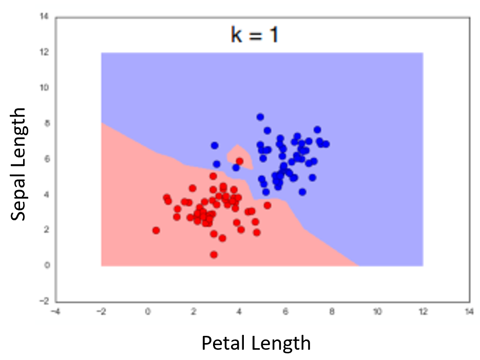
Note how we seem to have a bad point causing trouble.
Discussion
What difficulties or potential issues have we encountered?
Come up with theories of how that loner appeared?
How can we deal with such data points?
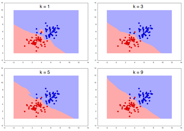
"$K$-Nearest-Neighbor" Algorithm - dealing with overfitting
As name implies, take vote of $K$ nearest samples to address those outliers.
Algorithm
The KNN algorithm is very simple to implement, as it does not need to be trained. The training phase merely stores the training data. For each test point, we calculate the distance of that data point to every existing data point and find the $K$ closest ones. What we return is the the most common amongst the top k classification nearest to the test point. Here's the pseudocode for K Nearest Neighbors:
kNN:

    Learn:
        Store training set T to X_train: X_train <-- T


    Predict:
        for every point xp in X_predict:
            for every point x in X_train:
                calculate the distance d in D between x and xp
            sort D in increasing order
            take the "k" items in X_train with the smallest distances to x
return the majority class among these k itemsDiscussion
K is a hyperparameter. How do we chose it?
How should we evaluate different possible K? What do we use to test?
Accuracy and Error Rate
We can assess the performance of a classifier by looking at the error rate and accuracy which are defined as follows. The error rate is the fraction of incorrect predictions over the testing set. Mathematically, we can express this as:
$$\text{Error Rate } = \frac{1}{n} \sum_{i=1}^n I(y_i \ne \hat{y}_i)$$
where $I$ is an indicator function that has the value $1$ when its argument is true, and $0$ otherwise.
Accuracy and Error Rate
$$\text{Error Rate } = \frac{1}{n} \sum_{i=1}^n I(y_i \ne \hat{y}_i)$$
The accuracy of a classifier is the fraction of correct predictions over the testing set:
$$\text{Accuracy } = \frac{1}{n} \sum_{i=1}^n I(y_i = \hat{y}_i) = 1 - \text{Error Rate}$$
Consider the accuracy on the training set versus a test set.
Lab
Compute accuracy for different values of K using training and test sets
Compare your algorithm to scikit version
manually run the classifier for the first data point and give prediction
Machine Learning Big Picture Again
Formal Problem: want to make a function or model $f$ that predicts the class label for a given input example ${\bf x}$, i.e. $\hat{y} = f({\bf x})$.
Step 1: Train the model. Need data $\bf x$ for which we know the label $y$ already. (preferrably a ton of these known ones). This is often called the training set. Find the best "$f$". This is called the Learning step.
Step 2. Because Machine learning methods love to overfit, we need to try the trained result from step 1 on some other known data and compare the estimated $f(\bf x)$ to the known $y$. Compute metrics and impress your boss/friends/reviewers. This is called Validation.
Step 3. Payoff time. Use it for something. Now we apply the data to some new $\bf x$ for which $y$ is unknown. Estimate the unknown $y$ by computing $f(\mathbf x)$. This is called Inference.
Quiz time
- Describe kNN algorithm in your own words
- what is k for?
- what is overfitting?
Loading the data
$$\hat{y} = f({\bf x})$$
- The value $\hat{y}$ belongs to a set $\{c_1,c_2,...,c_k\}$, each $c_i$ is a class label.
Data set for training or testing has inputs and known outputs so we can adjust $f$ to make it give the outputs we want it to.
$$ \mathcal{D} = \{ (\bf x_1, y_1), (\bf x_2, y_2), ... , (\bf x_k, y_k)\} $$ Up to you to decide how to best use it.
http://scikit-learn.org/stable/datasets/
Load one and find the inputs and outputs.
from sklearn.datasets import load_breast_cancer
ds = load_breast_cancer()
Train / Test Set Making in Scikit
http://scikit-learn.org/stable/modules/generated/sklearn.model_selection.train_test_split.html
Simply dividing the data in two parts.
from sklearn.model_selection import train_test_split


X_train, X_test, y_train, y_test = train_test_split(X, y, test_size=0.33, random_state=42)
KNeighborsClassifier in Scikit
http://scikit-learn.org/stable/modules/generated/sklearn.neighbors.KNeighborsClassifier.html
Methods
- fit(X, y) Fit the model using X as training data and y as target values
- get_params([deep]) Get parameters for this estimator.
- kneighbors([X, n_neighbors, return_distance]) Finds the K-neighbors of a point.
- kneighbors_graph([X, n_neighbors, mode]) Computes the (weighted) graph of k-Neighbors for points in X
- predict(X) Predict the class labels for the provided data
- predict_proba(X) Return probability estimates for the test data X.
- score(X, y[, sample_weight]) Returns the mean accuracy on the given test data and labels.
from sklearn.datasets import load_breast_cancer
ds = load_breast_cancer()
from sklearn.neighbors import KNeighborsClassifier

knn1 = KNeighborsClassifier(n_neighbors=1)
X = ds.data
y = ds.target
knn1.fit(X, y)
print(knn1.score(X,y))

knn1.fit(X_train, y_train)

print(knn1.score(X_train,y_train))
print(knn1.score(X_test,y_test))

print(knn1.score([X_test[0]],[y_test[0]]))

# which of these was cheating. Where are learning, validation, and inference done above?
X[0]
ds.target
General Scikit Use
import the module
from sklearn.neighbors import KNeighborsClassifierConstruct an instance of the class. Set hyperparameters here generally.
neigh = KNeighborsClassifier(n_neighbors=1)Fit mode to your dataset
neigh.fit(X_train, y_train)Extract desired information depending on method. These may be in attributes (see the method's doc page).