Outline
$Prob(X=x)$
Distributions
Gaussian a.k.a Normal distibution
Conditional probability
Bayes Law
Naive Bayes Classification
import numpy as np
from matplotlib import pyplot as plt
%matplotlib inline
Randomness
Random variable $X$ - a variable whose measured value can change from one replicate of an experiment to another. E.g., the unknown coin flip result.
"Range of $X$" = values it can take, a.k.a. outcomes. E.g., $\{HEADS, TAILS\}$.
New kind of notation $P(X=x)$ aka $Prob(X=x)$ is probability that the random variable $X$ will take the value of $x$ in an experiment.
E.g., $P(\text{coin flip result} = HEADS)$
$P(\text{"event"})$ can be very abstract, such as $P(X\le 5)$ or $P(X\le 5, X\ge 2)$.
How does relate to the statisticians' "sample"?
Probability
A probability $P(\text{"event"})$ is a number between 0 and 1 representing how likely it is that an event will occur.
Probabilities can be:
Frequentist: $\frac{number \ of \ times \ event \ occurs}{number \ of \ opportunities \ for \ event \ to \ occur}$
Subjective: represents degree of belief that an event will occur
e.g. I think there's an 80% chance it will be sunny today $\rightarrow$ P(sunny) = 0.80
The rules for manipulating probabilities are the same, regardless how we interpret probabilities.
New Concepts
Probability $P(X=x)$
Distribution - a theoretical version of a histogram:
- Expectation $E(\cdot )$ - a theoretical version of a mean: $ \bar{x} \rightarrow E(x) $
Discrete Distribution - Probability Mass Function $f(x_i) = P(X = x_i)$
Remember $f(x_i)$ aren't values we measure, they're probabilities for values we measure (or relative frequencies).
** So scale histogram by total to make numbers relative for distribution.
Exercise
We flip a coin 100 times and get 60 heads and 40 tails.
- What is (apparently) $P(X=HEADS)$ and $P(X=TAILS)$?
- What might the distribution look like?
Expectation: Mean & Variance, Revisited
Recall, for a statistical population, when $x_i$ were independent samples: \begin{align} \text{Population mean} &= \mu = \frac{\sum_{i=1}^N x_i}{N} \\ \text{Population variance} &= \sigma^2 = \frac{\sum_{i=1}^N (x_i - \mu)^2}{N} \\ \end{align}
For a random variable $X$, for which all possible values are $x_1$, $x_2$,... $x_N$: \begin{align} \text{Mean} &= \mu = E(X) = \sum_{i=1}^N x_i f(x_i) \\ \text{Variance} &= \sigma^2 = V(X) = E(X-\mu^2) = \sum_{i=1}^N x_i^2 f(x_i) - \mu^2 \\ \end{align}
Theoretical way to accomplish the same thing by adding them up smarter.
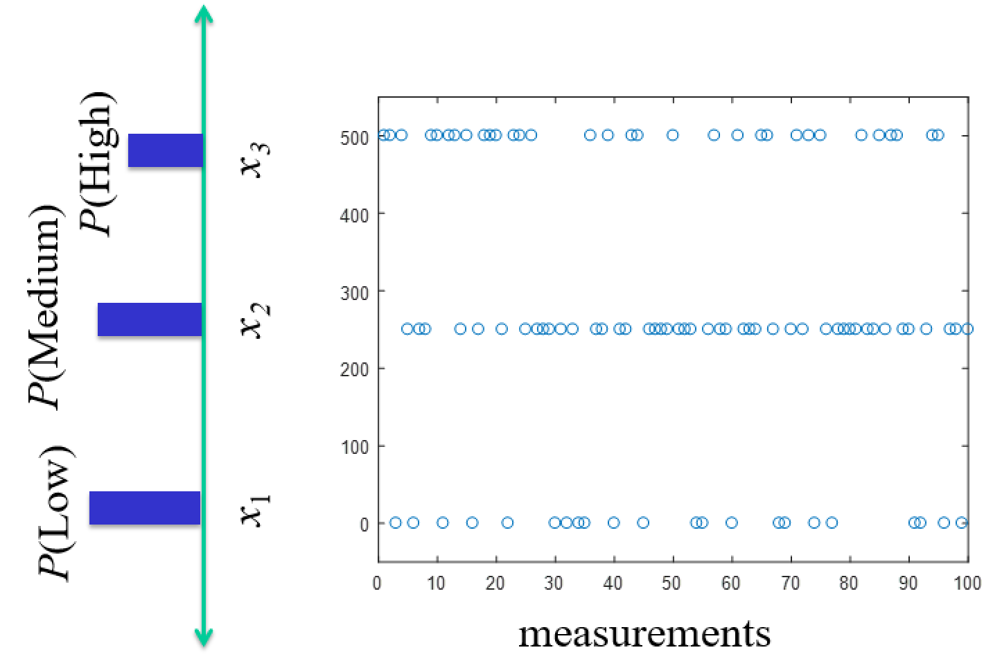
Three-sided example $x_1=0,x_2=1,x_3=2$
Samples are: 1, 0, 2, 0, 1, 0, 1, 1, 2, 0, 1
So what are the relative frequencies of $x_1$, $x_2$, and $x_3$?
What is sample mean?
What is $E[X]$ using formula?
Three-sided example $x_1=0,x_2=1,x_3=2$
Samples are: 1, 0, 2, 0, 1, 0, 1, 1, 2, 0, 1
\begin{align} \text{Population mean} &= \mu = \frac{\sum_{i=1}^N x_i}{N} \\ &= \frac{1}{11}(1 + 0 + 2 + 0 + 1 + 0 + 1 + 1 + 2 + 0 + 1)1 \text{, for a population of 11 } \\ &= \frac{1}{11}(0+0+0+0) + \frac{1}{11}(1+1+1+1+1) + \frac{1}{11}(2+2)\\ &= \frac{1}{11} 4\times 0 + \frac{1}{11} 5\times 1 + \frac{1}{11} 2 \times 2 \\ &= \frac{4}{11} \times 0 + \frac{5}{11} \times 1 + \frac{2}{11} \times 2 \\ &\approx f(x_1) x_1 + f(x_2) x_2 + f(x_3) x_3 \text{ the relative frequency} \end{align}
\begin{align} \text{Mean, a.k.a. Expected value} &= \mu = E(X) = \sum_{i=1}^N x_i f(x_i) \\ \end{align}
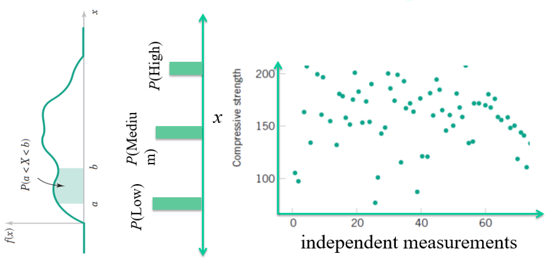
Continuous Distributions - Probability Density Function $f(x) = P(X = x)$
Essentially just the continuous limit. Sums $\rightarrow$ integrals.
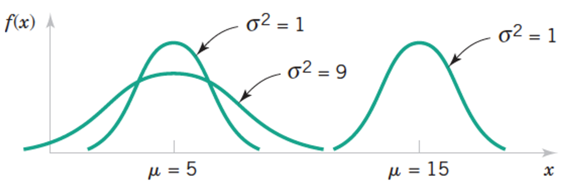
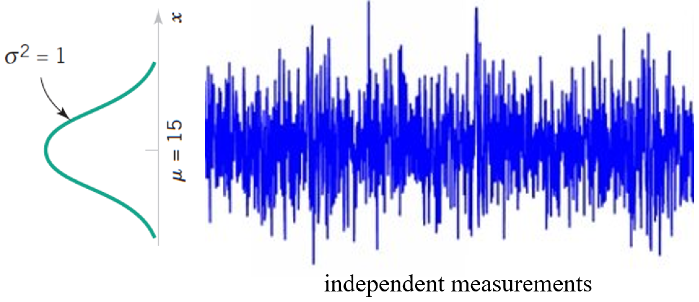
The Normal Distribution
- Most widely-used model for the distribution of a random variable
- Central limit theorem (good approximation to most situations)
- Also known as Gaussian distribution
$$ f(x) = \frac{1}{\sqrt{2\pi}\sigma} e^{\frac{-(x-\mu)^2}{2\sigma^2}} \text{ for } -\infty < x < \infty $$
\begin{align} E(X) &= \mu \\ V(X) &= \sigma^2 \end{align}
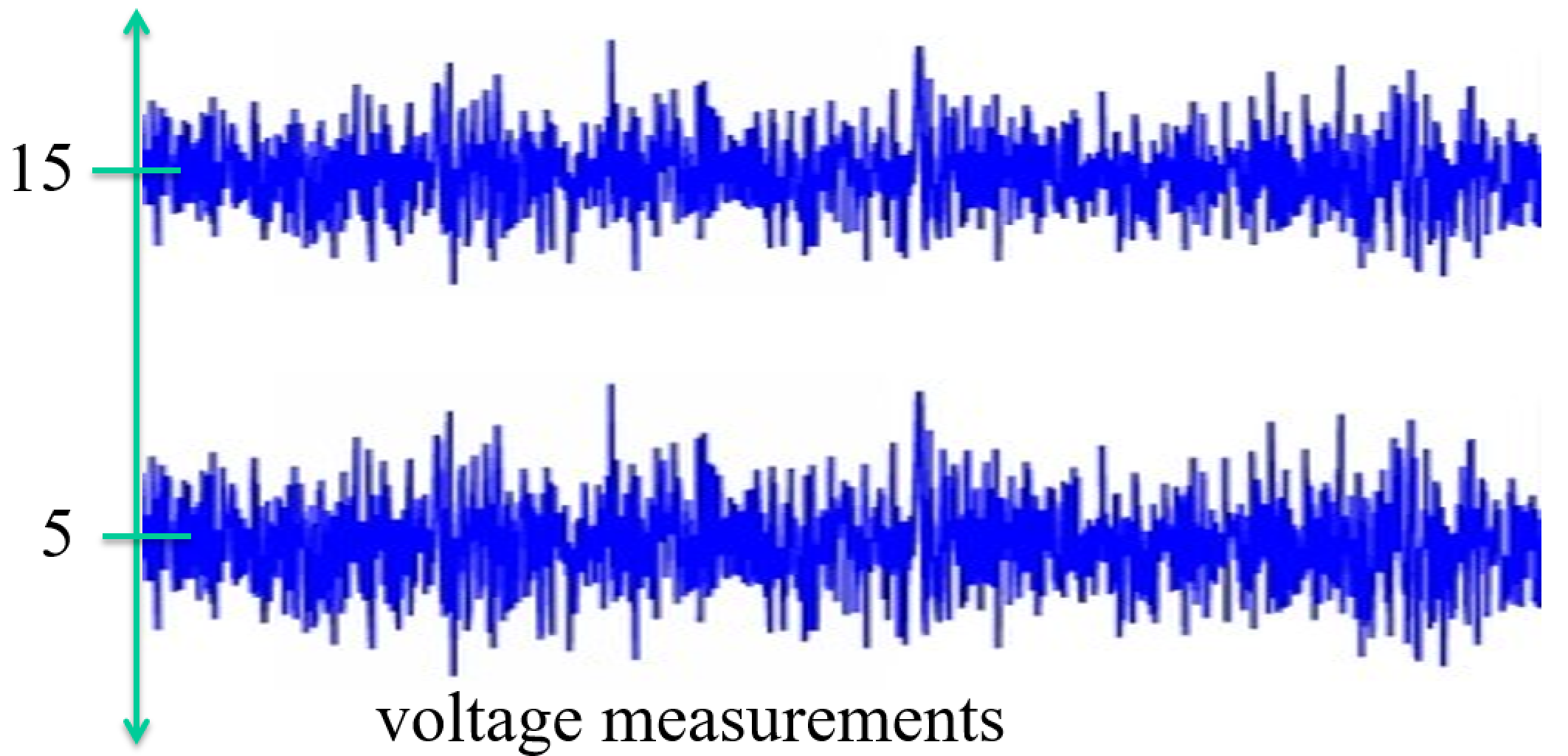
The Normal Distribution $X \sim N(\mu, \sigma)$
$$ f(x) = \frac{1}{\sqrt{2\pi}\sigma} e^{\frac{-(x-\mu)^2}{2\sigma^2}} \text{ for } -\infty < x < \infty $$
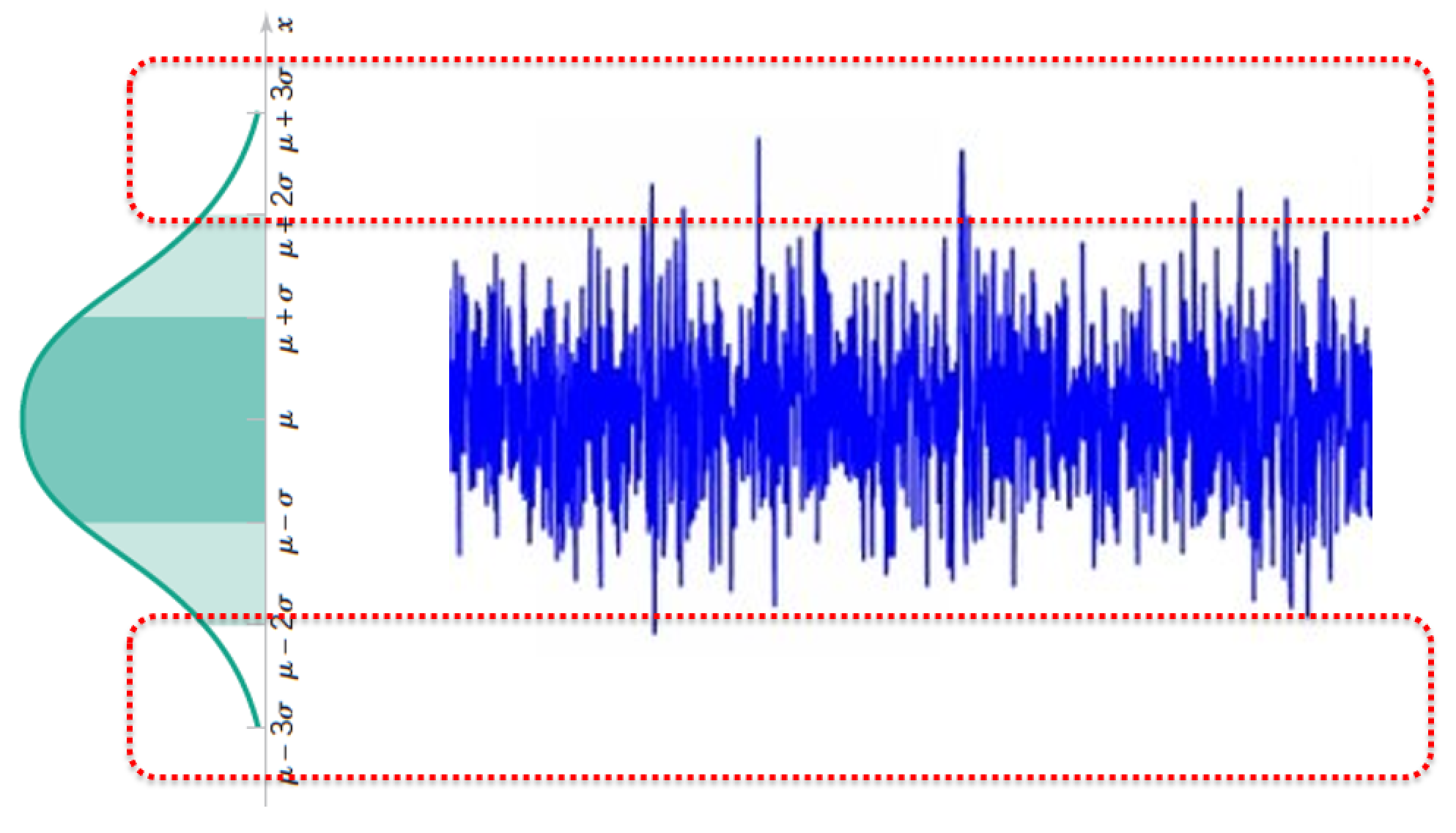
Tails of the Normal Distribution $X \sim N(\mu, \sigma)$
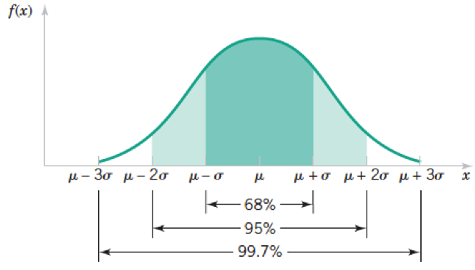
Tails of the Normal Distribution $X \sim N(\mu, \sigma)$
The Standard Normal Distribution $Z$
- If $X$ is a normal r.v. with $E(X) = \mu$ and $V(X) = \sigma^2$
$$ Z = \frac{X-\mu}{\sigma} $$
- $Z$ is a normal r.v. with $E(X) = 0$ and $V(X) = 1$
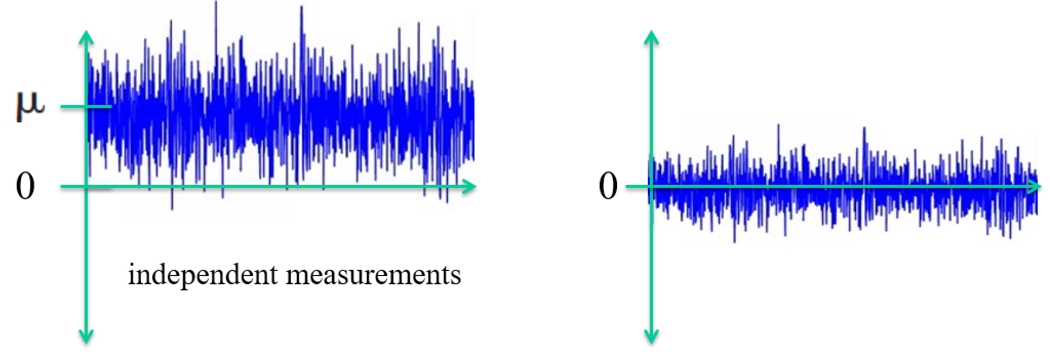
- "Standardizing" the data
Exercise
Load a dataset and compute mean and variance of a column
Standardize the column
Now compute mean and variance of the result
Tricky Exercise
Consider a $m \times 3$ matrix $\mathbf A$ with columns $\mathbf x, \mathbf y$, and $\mathbf z$ (each a vector of data).
Suppose we standardize the three columns to make $\bar{\mathbf A}$.
What are the elements of $\bar{\mathbf A}^T \bar{\mathbf A}$?
Part 2. Conditional Probability and Bayes Law
Problem
You have a database of 100 emails.
- 60 of those 100 emails are spam
- 48 of those that are spam have the word "buy"
- 12 of those that are spam don't have the word "buy"
- 40 of those 100 emails aren't spam
- 4 of those that aren't spam have the word "buy"
- 36 of those that aren't don't have the word "buy"
What is the probability that an email is spam?
What is the probability that an email is spam if it has the word "buy"?
(Draw a Venn diagram.)
Solution
There are 48 emails that are spam and have the word "buy". And there are 52 emails that have the word "buy": 48 that are spam plus 4 that aren't spam. So the probability that an email is spam if it has the word "buy" is 48/52 = 0.92
If you understood this answer then you have understood the Bayes Theorem (in a nutshell).
Joint Probability
Consider two of our abstract "events" $A$ & $B$.
How do we mathematically write the new event consisting of both events.
Ex.
- expeimental measurement $X\le 5$ and $X\ge 2$
- email is spam and email contains word "buy"
- coin flip #1 is HEADS and coin flip #2 is HEADS
Draw diagrams that explain the possible combinations.
Joint Probability
A. we characterize the intersection of events with the joint probability of $A$ and $B$, written $P(A \cap B)$.
$P(A) =$ probability of being female
$P(B) =$ probability of having long hair
$P(A \cap B)$ = the probability of being female AND having long hair
We might also write $P(A \text{ and } B)$
Most-commonly written as just $P(A, B)$. Both events happenning implies intersection.
Conditional Probability
Suppose event $B$ has occurred. What quantity represents the probability of $A$ given this information about $B$?
- Probability someone is female given that they have long hair
- Probability that someone has long hair given that they are female
This is called the conditional probability of $A$ given $B$ - the probability that event A occurs, given that event B has occurred.
It is written $P(A\,|\,B)$. Read $P(A\,|\,B)$ as "probability of $A$, given $B$".
We already solved an example of this: $P$(email is spam | has the word "buy")
Another: probability a coin toss will be HEADS given that prior coin toss was HEADS?
Thinking Lab
Can you guess the (abstract) relationship between $P(A\,|\,B)$ and $P(A\cap B)$?
Return to your spam diagram and results.
Conditional Probability
Q. Suppose event $B$ has occurred. What quantity represents the probability of $A$ given this information about $B$?
A. The intersection of $A$ & $B$ divided by region $B$.
This is called the conditional probability of $A$ given $B$ - the probability that event A occurs, given that event B has occurred.
It is written $P(A\,|\,B)$, and is given by
$$ P(A\,|\,B) = \frac{P(A\cap B)}{P(B)} $$
Notice, with this we can also write $P(A \cap B) = P(A\,|\,B) \times P(B)$.
More on Conditional Probability
- Conditioning on event $B$ means changing the sample space to $B$
- Think of $P(A|B)$ as the chance of getting an $A$, from the set of $B$'s only
The symbol $P(\ \ |B)$ should behave exactly like the symbol $P$
For example,
$$P(C \cup D) = P(C) + P(D) - P(C \cap D)$$
$$P(C \cup D|B) = P(C|B) + P(D|B) - P(C \cap D|B)$$
Independent Events
Events A and B are independent if and only if: $$P(A \cap B) = P(A)P(B)$$
Equivalently,
$$ P(A\,|\,B) = P(A) $$ $$ P(B\,|\,A) = P(B) $$
Draw a diagram representing this situation.
Think of a good example.
Can you guess what "disjoint events" would mean? Are they independent?
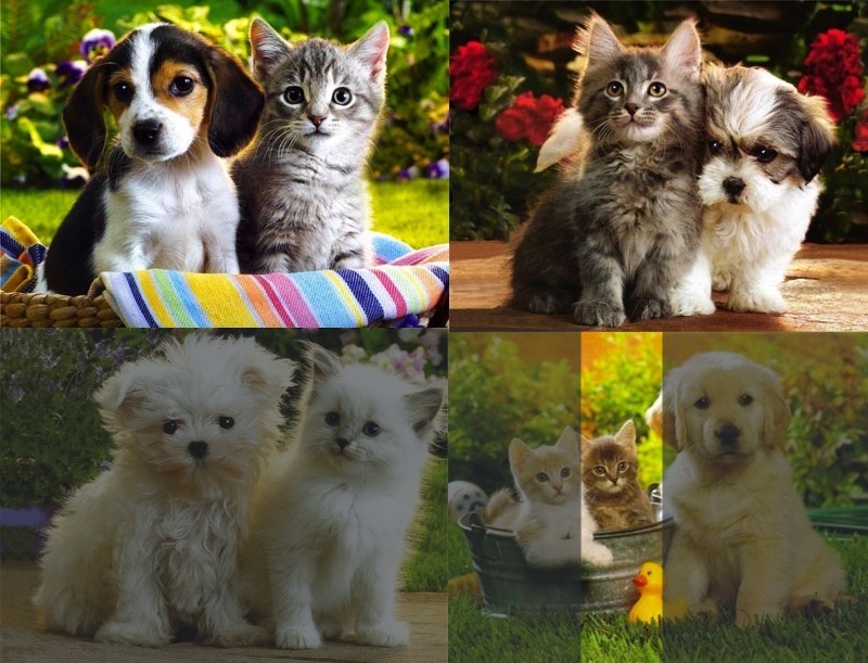
Exercises: Probability with the help of small animals
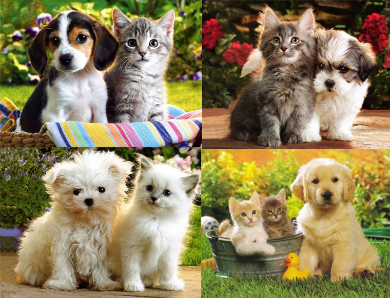
- If we randomly pick one small animal, what is the probablity that we get a puppy? $P(\text{puppy})$
- If we randomly pick one small animal, what is the probablity that it is dark-colored? $P(\text{dark fur})$
- Given that we picked a dark-colored animal, what is the probability that it is a puppy? (use equation)
Q: If we randomly pick one small animal, what is the probablity that we get a puppy?
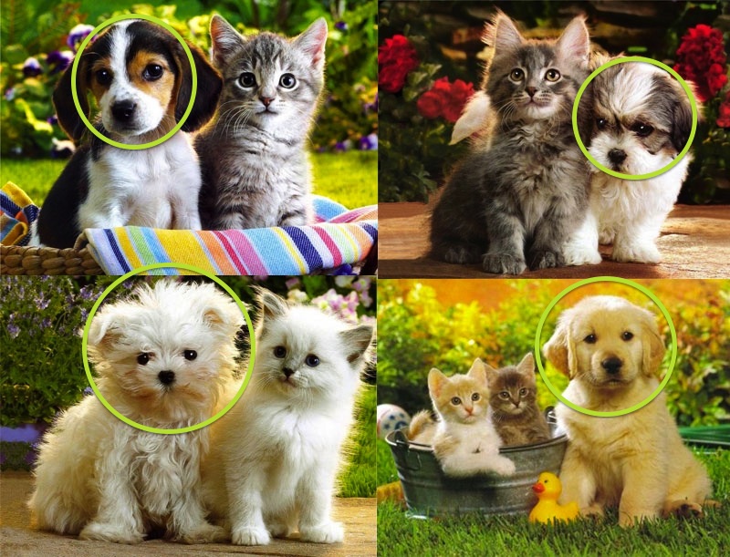
$P(puppy) = 4/9$
Q: If we randomly pick one small animal, what is the probablity that it is dark-colored?
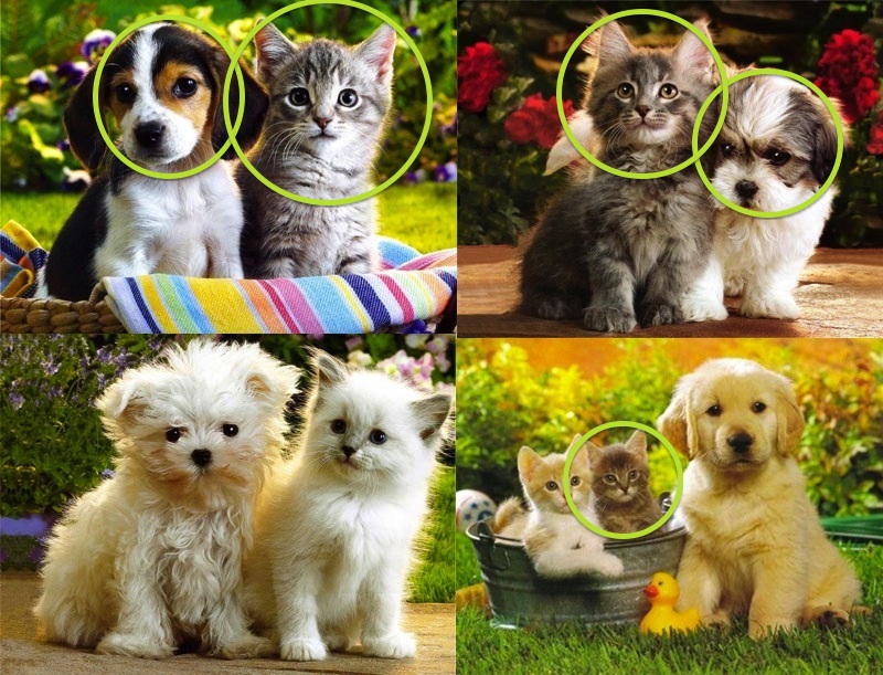
$P(dark) = 5/9$
Q: Given that we picked a dark-colored animal, what is the probability that it is a puppy?
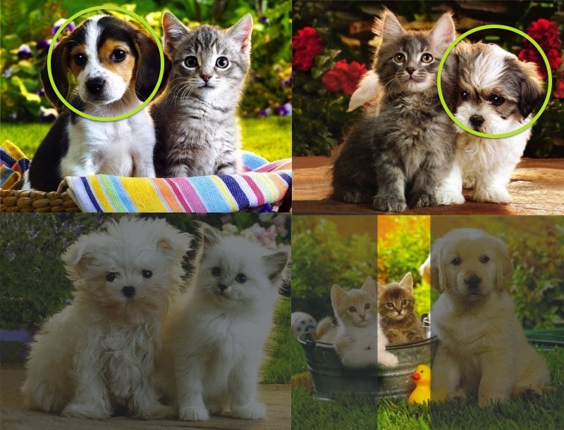
$P(puppy|dark) = \frac{P(\text{dark } \cap \text{ puppy})}{P(\text{dark})} = \frac{^2/_9}{^5/_9} = \frac{.222}{.556} = .4$
The Law of Total probability - Complete Partition of Outcomes
Motivation: we wish to go backwards and get the marginal probability $P(A)$ from $P(A\,|\,B_1),P(A\,|\,B_2),...,P(A\,|\,B_n)$.
Reconsider the Venn diagram. Suppose we know the conditional probabilities for a set of events, $B_1$, $B_2$, ..., $B_n$, which forms a complete partitioning of possible outcomes (so they are disjoint).
Examples:
- $B_1$ = HEADS, $B_2$ = TAILS.
- $B_1$ = Disease, $B_2$ = Healthy.
- $B_1$ = dog, $B_2$ = not-a-dog.
Note in two-partition case, $B_2 = B_1^c$. What is $P(B_1^c)$ using $P(B_1)$?
Total probability
If $B_1, B_2, \dots, B_k$ form a partition of $\Omega$, then $(A \cap B_1), (A \cap B_2), \dots, (A \cap B_k)$ form a partition of the set or event A.
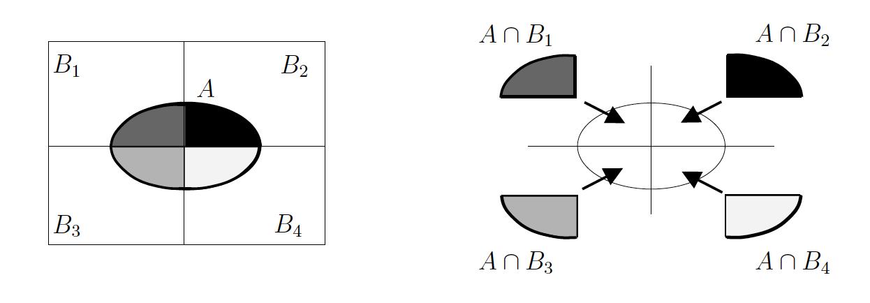
The probability of event A is therefore the sum of its parts:
$$P(A) = P(A \cap B_1) + P(A \cap B_2) + P(A \cap B_3) + P(A \cap B_4)$$
Total probability
If $B_1, \dots, B_n$ partition possible outcomes, then for any event A, we can add up the intersections to get $P(A)$
$$ P(A) = \sum_{i = 1}^n P(A \cap B_i)$$
Recall conditional probability is:
$$ P(A|B) = \frac{P(A\cap B)}{P(B)} $$
Combine these equations to derive a relation between $P(A)$ and $P(A\,|\,B)$.
Law of Total probability
Hopefully everyone believes...
If $B_1, \dots, B_n$ partition possible outcomes, then for any event A, we can add up the intersections to get $P(A)$
$$ P(A) = \sum_{i = 1}^n P(A \cap B_i)$$
So plugging in $P(A \cap B) = P(A|B) \times P(B)$, gives us:
$$ P(A) = \sum_{i = 1}^n P(A \cap B_i) = \sum_{i = 1}^n P(A | B_i) P(B_i) $$
Exercise:
Tom gets the bus to campus every day. The bus is on time with probability 0.6, and late with probability 0.4. The buses are sometimes crowded and sometimes noisy, both of which are problems for Tom as he likes to use the bus journeys to do his Stats assignments. When the bus is on time, it is crowded with probability 0.5. When it is late, it is crowded with probability 0.7. The bus is noisy with probability 0.8 when it is crowded, and with probability 0.4 when it is not crowded.
Formulate events C and N corresponding to the bus being crowded and noisy. Do the events C and N form a partition of the sample space? Explain why or why not.
Write down probability statements corresponding to the information given above. Your answer should involve two statements linking C with T and L, and two statements linking N with C. (T = "on time", L = "late")
Find the probability that the bus is crowded.
Find the probability that the bus is noisy.
- Let $C = “crowded”$, $N =“noisy”$. $C$ and $N$ do NOT form a partition of the sample space. It is possible for the bus to be noisy when it is crowded, so there must be some overlap between $C$ and $N$.
- $P(T) = 0.6$; $P(L) = 0.4$; $P(C | T) = 0.5$; $P(C | L) = 0.7$; $P(N | C) = 0.8$; $P(N | C^c) = 0.4$.
- $P(C) = P(C | T)P(T) + P(C | L)P(L) = 0.5 \times 0.6 + 0.7 \times 0.4 = 0.58$
- $P(N) = P(N | C)P(C) + P(N | C^c)P(C^c) = 0.8 \times 0.58 + 0.4 \times (1 - 0.58) = 0.632$
Bayes' Theorem a.k.. Bayes Law
Objective: relate $P(A\,|\,B)$ to $P(B\,|\,A)$.
Motivation 1 - Inverse problems: $P(B\,|\,A)$ easy to get, $P(B\,|\,A)$ difficult.
E.g. $A$ = disease, $B$ = symptom.
- $P(\text{symptom} \,|\, \text{disease})$ is well-known, textbook info.
- $P(\text{disease} \,|\, \text{symptom})$ depands on all the other possible causes. As well as the prior probability of that particular cause.
Bayes' Theorem a.k.. Bayes Law
Objective: relate $P(A\,|\,B)$ to $P(B\,|\,A)$.
Motivation 2 - Tricky / non-intuitive situations. (trust-the-math time).
Rare events:
- Probability you have a rare disease given you test positive. Ex.: False positive rate for test is 2 percent, but 0.01 percent of people have disease. Which is more likely, you got a false positive or you have the disease? Answer: False positive.
- Probability someone is a terrorist given that they fit the profile.
Key factor again: prior probability
Bayes' Theorem a.k.. Bayes Law
Objective: relate $P(A\,|\,B)$ to $P(B\,|\,A)$.
We can derive the relationship using our Eq. for Conditional Probability...
\begin{align} P(A \cap B) &= P(A\,|\,B) \times P(B)\qquad \\ P(B \cap A) &= P(B\,|\,A) \times P(A)\qquad \text{ by substitution} \end{align}
And we know that $P(A \cap B) = P(B \cap A)\qquad$
$\Rightarrow P(A\,|\,B) \times P(B) = P(B\,|\,A) \times P(A)\>$ by combining the above
$\Rightarrow P(A\,|\,B) = \frac{P(B\,|\,A) \times P(A)}{P(B)}\>$ by rearranging last step
This result is called Bayes’ theorem. Here it is again:
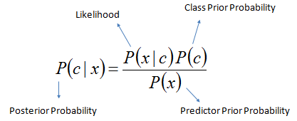
$$ P(A\,|\,B) = \frac{P(B\,|\,A) \times P(A)}{P(B)} $$
$P(A\,|\,B)$ is the posterior probability. E.g. $P(\text{disease} \,|\, \text{symptom})$
$P(B\,|\,A)$ is the likelihood. E.g. $P(\text{symptom} \,|\, \text{disease})$
$P(A)$ is the prior probability. E.g. $P(\text{disease})$, the overall rarity.
$P(B)$ is the evidence. E.g. $P(\text{symptom})$, evidence suggesting disease.
Wikipedia has a lot on Bayes: https://en.wikipedia.org/wiki/Bayes_theorem
By law of total probability,
$$ P(A\,|\,B) = \frac{P(B\,|\,A) \times P(A)}{P(B)} = \frac{P(B\,|\,A) \times P(A)}{P(B\,|\,A) \times P(A) + P(B\,|\,A^c) \times P(A^c)} $$
Big Exercise
Suppose a disease infects one out of every 1000 people in a population...
and suppose that there is a good, but not perfect, test for this disease:
- If a person has the disease, the test is positive 99% of the time.
- On the other hand, the test also produces some false positives. About 2% of uninfected patients also test positive.
You just tested positive. What are your chances of having the disease?
| A | not A | sum | |
|---|---|---|---|
| B | $P(A\cap B)$ | $P(A^c \cap B)$ | $P(B)$ |
| not B | $P(A \cap B^c)$ | $P(A^c \cap B^c)$ | $P(B^c)$ |
| $P(A)$ | $P(A^c)$ | $1$ |
$ P(A \cap B) = P(B|A)P(A) = (.99)(.001) = .00099 $
$ P(A^c \cap B) = P(B|A^c)P(A^c) = (.02)(.999) = .01998 $
Let's fill in some of these numbers:
| A | not A | sum | |
|---|---|---|---|
| B | $.00099$ | $.01998$ | $.02097$ |
| not B | $P(A \cap B^c)$ | $P(A^c \cap B^c)$ | $P(B^c)$ |
| $.001$ | $.999$ | $1$ |
arithmetic gives us the rest:
| A | not A | sum | |
|---|---|---|---|
| B | $.00099$ | $.01998$ | $.02097$ |
| not B | $.00001$ | $.97902$ | $.98903$ |
| $.001$ | $.999$ | $1.0$ |
From which we directly derive:
$$ P(A|B) = \frac{P(A \cap B)}{P(B)} = \frac{.00099}{.02097} = .0472 $$
From which we directly derive:
$$ P(A|B) = \frac{P(A \cap B)}{P(B)} = \frac{.00099}{.02097} = .0472 $$
FYI: Chain Rule for Probability
It just keeps going...
We can write any joint probability as incremental product of conditional probabilities,
$ P(A_1 \cap A_2) = P(A_1)P(A_2 \,|\, A_1) $
$ P(A_1 \cap A_2 \cap A_3) = P(A_1)P(A_2 \,|\, A_1)P(A_3 \,|\, A_2 \cap A_1) $
In general, for $n$ events $A_1, A_2, \dots, A_n$, we have
$ P (A_1 \cap A_2 \cap \dots \cap A_n) = P(A_1)P(A_2 \,|\, A_1) \dots P(A_n \,|\, A_{n-1} \cap \dots \cap A_1) $
Part 3. Naive Bayes Classification
Naive Bayes Motivation
Popular for text (perhaps exclusively)
Still works when have many many features, and perhaps less samples
Can handle streaming and massive data (i.e., many samples too)
Text classification problem. We have the text of documents and would like to classify their topic (e.g. sports, politics, arts, etc.), or perhaps classify emails as spam or not (ham).
Consider using KNN for this. Imagine have 1B spam emails and 10M ham.
Naive Bayes approach: use that giant database as training to compute conditional probabilities which describe spam (training step). Then just use those conditional probabilities to classify new emails (inference step).
References
- https://en.wikipedia.org/wiki/Naive_Bayes_classifier
- https://www.youtube.com/watch?v=M59h7CFUwPU - Udacity video on NB
- https://www.youtube.com/watch?v=ajG5Yq1myMg - Video of calculation details
- http://www.cs.columbia.edu/~mcollins/em.pdf - Naive Bayes and EM method for building models without labels
Using Bayes Law for Classification: Step I. Problem Formulation.
Suppose we want to classify documents as being one of: sports, politics, art.
We want to use the words it contains to estimate the probability of belonging to each category.
- What are the "events"?
- What are the conditional probabilities here?
Using Bayes Law for Classification: Step II. Computing Terms.
Suppose we have a large number of labeled examples. How do we use it to estimate these terms?
- $P(\text{word_x})$
- $P(\text{topic_y})$
- $P(\text{word_x}\,|\,\text{topic_y})$
Hint: frequentist interpretation of probabilities.
Exercise
We have 8 articles in our dataset:
- 3 sports articles
- 4 politics articles
- 1 arts article
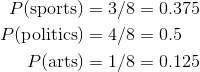
What are $P(\text{sports})$, $P(\text{politics})$, $P(\text{arts})$? Which terms are these in the Bayes Law equation?
Priors
The priors are the likelihood of each class. Based on the distribution of classes in our training set, we can assign a probability to each class:
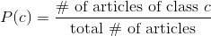
Take a very simple example where 3 classes: sports, news, arts. There are 3 sports articles, 4 politics articles and 1 arts articles. This is 8 articles total. Here are our priors:
Exercise
Let's look at the word "ball". Here are the occurrences in each of the 8 documents. We also need the word count of the documents.
| Article | Occurrences of "ball" | Total # of words |
|---|---|---|
| Sports 1 | 5 | 101 |
| Sports 2 | 7 | 93 |
| Sports 3 | 0 | 122 |
| Politics 1 | 0 | 39 |
| Politics 2 | 0 | 81 |
| Politics 3 | 0 | 142 |
| Politics 4 | 0 | 77 |
| Arts 1 | 2 | 198 |
Which terms in the Bayes Law equation can we calulate with this info?
Do the calculation.
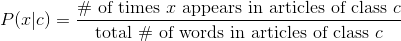
Conditional Probability Table
The first step is building the Conditional Probability Table (CPT). We would like to get, for every word, the count of the number of times it appears in each class. We are calculating the probability that a random word chosen from an article of class c is word x.
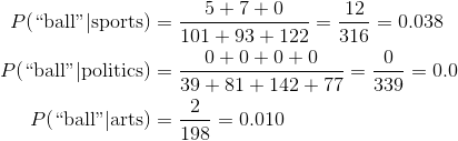
Again, let's take our example. Let's look at the word "ball". Here are the occurrences in each of the 8 documents. We also need the word count of the documents.
| Article | Occurrences of "ball" | Total # of words |
|---|---|---|
| Sports 1 | 5 | 101 |
| Sports 2 | 7 | 93 |
| Sports 3 | 0 | 122 |
| Politics 1 | 0 | 39 |
| Politics 2 | 0 | 81 |
| Politics 3 | 0 | 142 |
| Politics 4 | 0 | 77 |
| Arts 1 | 2 | 198 |
Here are the values in the CPT table for the word "ball". We will do these calculations for all the words that appeared in the training documents.
Using Bayes Law for Classification: Step II. Computing Terms (cont.)
Now we wish to use a bunch of words to improve performance. So how would we compute:
$$P(\text{word_1 and word_2 and ... and word_n}\,|\,\text{topic_y})$$
Suppose $n=1000$. How many different terms would that require we compute?
The Naive Assumption of Naive Bayes
A universal problem with using Bayesian methods in high dimensions is variable dependence. In general data will have complex structure in the relationships between variables.
An almost-equally-universal tactic when using Bayesian mathods is to ignore the structure and presume independence between variables. In which case we can make the following approximation:
$$P(\text{word_1 and word_2 and ... and word_n}\,|\,\text{topic_y}) = ?$$
Naivete of Naive Bayes
We make a BIG assumption here that the occurrences of each word are independent. If they weren't, we wouldn't be able to just multiply all the individual word probabilities together to get the whole document probability. Hence the "Naive" in Naive Bayes.
Take a moment to think of how absurd this is. A document that contains the word "soccer" is probably more likely to contain the word "ball" than an average document. We assume that this is not true! But it turns out that this assumption doesn't hurt us too much and we still have a lot of predictive power. But the probabilities that we end up with are not at all true probabilities. We can only use them to compare which of the classes is the most likely.
Pro-tip: you can reduce this error by removing redundant variables (e.g. words that highly correlate with other words).
Exercise
Estimate $P(\text{"ball" and "state"}\,|\,\text{topic})$ for all three topics:
| Article | "ball" | "state" | Total words |
|---|---|---|---|
| Sports 1 | 5 | 2 | 101 |
| Sports 2 | 7 | 0 | 93 |
| Sports 3 | 0 | 0 | 122 |
| Politics 1 | 0 | 8 | 39 |
| Politics 2 | 0 | 2 | 81 |
| Politics 3 | 0 | 1 | 142 |
| Politics 4 | 0 | 0 | 77 |
| Arts 1 | 2 | 0 | 198 |
Zero Probabilities
If a word has never before appeared in a document of a certain class, the probability will be 0. Since we are multiplying the probability, the whole probability becomes 0! We basically lose all information.
In the above example, since "ball" never appears in a politics article in the training set, if it appeared in a new article, we would say that there was a 0% chance that that was a politics article. But that's too harsh!
How can we fix this?
Laplace Smoothing
The simplest option is to replace these zeros with a really small value, like 0.00000001. The better option is Laplace Smoothing.
Laplace Smoothing is assuming that every word has been seen by every article class one extra time.
Here's our new conditional probability with Laplace smoothing.
$$P(x|c) = \frac{\text{(# times word $x$ appears in articles of class c) + 1}}{(\text{total # words in articles of class c)}}$$
The standard is to use 1 as the smoothing constant, but we could assume every word appeared a fraction of a time, using a smoothing constant $\alpha$ which we can tune, in place of "1".
Exercise
Calculate $P(\text{sports} \,|\, \text{"ball" and "state"})$.
Summary of Naive Bayes Algorithm
- Training: Calculate the priors and Conditional Probability Table
- Predict: Calculate the probabilities for the new article for each label and pick the max
One Bayes, many models
- Multinomial Bayes (what we did above, by just using relative frequencies)
- Bernoulli Bayes
- Gaussian Bayes
Flexibility of Application:
In theory you can use any prior distribution and any distribution for each feature. This makes it quite adaptable and allows a data scientist to easily incorporate domain knowledge.
Lab
Load the "20newsgroups" dataset in sklearn and run the built-in Naive Bayes classifier.
#from sklearn.datasets import fetch_20newsgroups

#ng20 = fetch_20newsgroups()
#dir(ng20)
#ng20.target_names
#ng20.target
#ng20.data[0]
Log Likelihood
These probability values are going to get really small. Theoretically, this is not an issue, but when a computer makes the computation, we run the risk of numerical underflow. To keep our values bigger, we take the log. Recall that this is true: log(ab) = log(a) + log(b)
The MLE is written:

Recall that if a > b log(a) > log(b) so we can still find the maximum of the log likelihoods.