Outline
Projects
The "Art" of optimization
Maximum Likelihood
MAP Estimation
import numpy as np
from matplotlib import pyplot as plt
%matplotlib inline
Projects
Requirements:
- Must be python, delivered in Jupyter notebook.
- Must be supervised learning problem.
Preliminary Rubric:
- Data selection interesting/challenging?
- Method interesting/challenging/thorough?
- Validation thorough, done properly?
- Report - well-written/understandable, explains pros/cons of method, what happened & why (can use jupyter completely if use markdown & latex).
Note: some related tasks will go into participation or homework grade.
Optimization
A framework for describing problems for minimizing/maximizing functions Plus an "art" for finding easier alternative problems that have same minimizer.
\begin{align} \text{minimizer: } \mathbf z^* &= \arg\min\limits_{\mathbf z} g(\mathbf z) \\ \text{minimum: } g_{min} &= \min\limits_{\mathbf z} g(\mathbf z) = g(\mathbf z^*) \end{align}
What is "$g$" and $\mathbf z$ for our regression problem? for KNN? Naive Bayes?
Note 1: nuanced jargon here, minimizer is location of minimum, not minimum value itself.
Note 2: we aren't concerned with local vs. global minima. But know they differ.
The "Art" of Optimization
Find minimizer for $p(\mathbf z) + q$, where $q$ is a constant, by minimizing... what?
Find maximizer for $g(\mathbf z)$ by minimizing... what?
Finding the minimizer for the Euclidean norm $\Vert \mathbf v \Vert$ is tricky, since it isn't smooth. What's a smooth function we could minimize instead to easily solve the problem?
How about the maximizer for $\exp\big(-\frac{1}{2 \sigma^2} \Vert \mathbf z - \mathbf z_0 \Vert^2 \big)$?
Maximum Likelihood Estimation
Recall the system (what is it?): $\mathbf y = \mathbf X \boldsymbol\beta + \boldsymbol\varepsilon$.
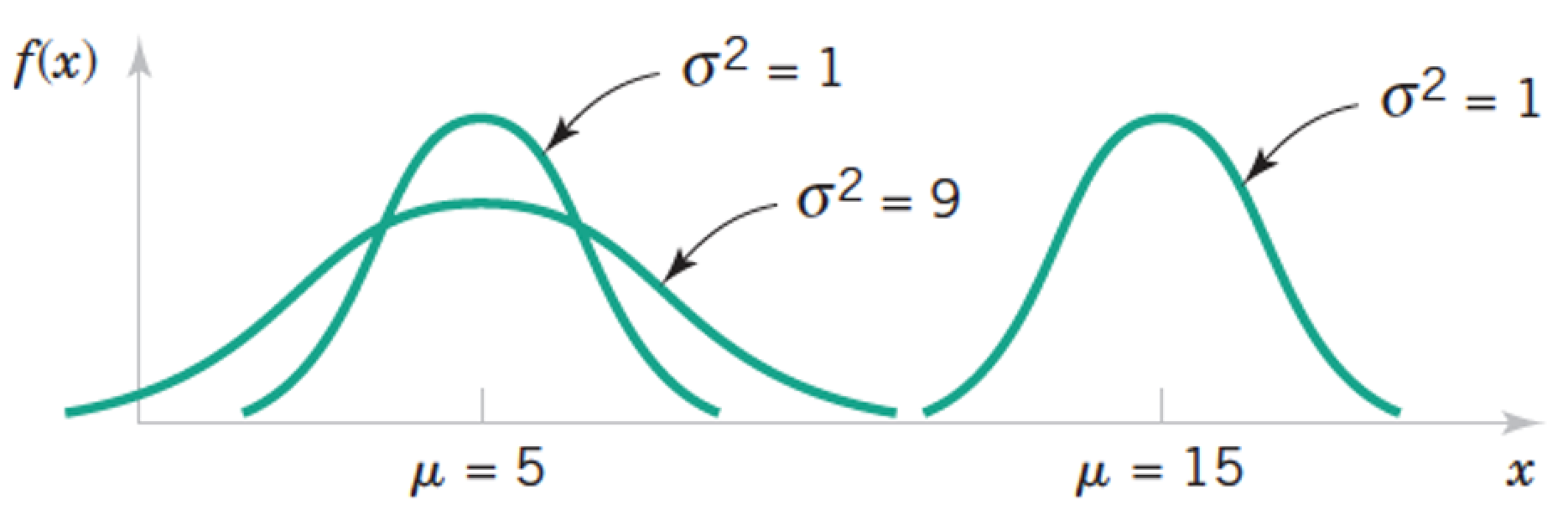
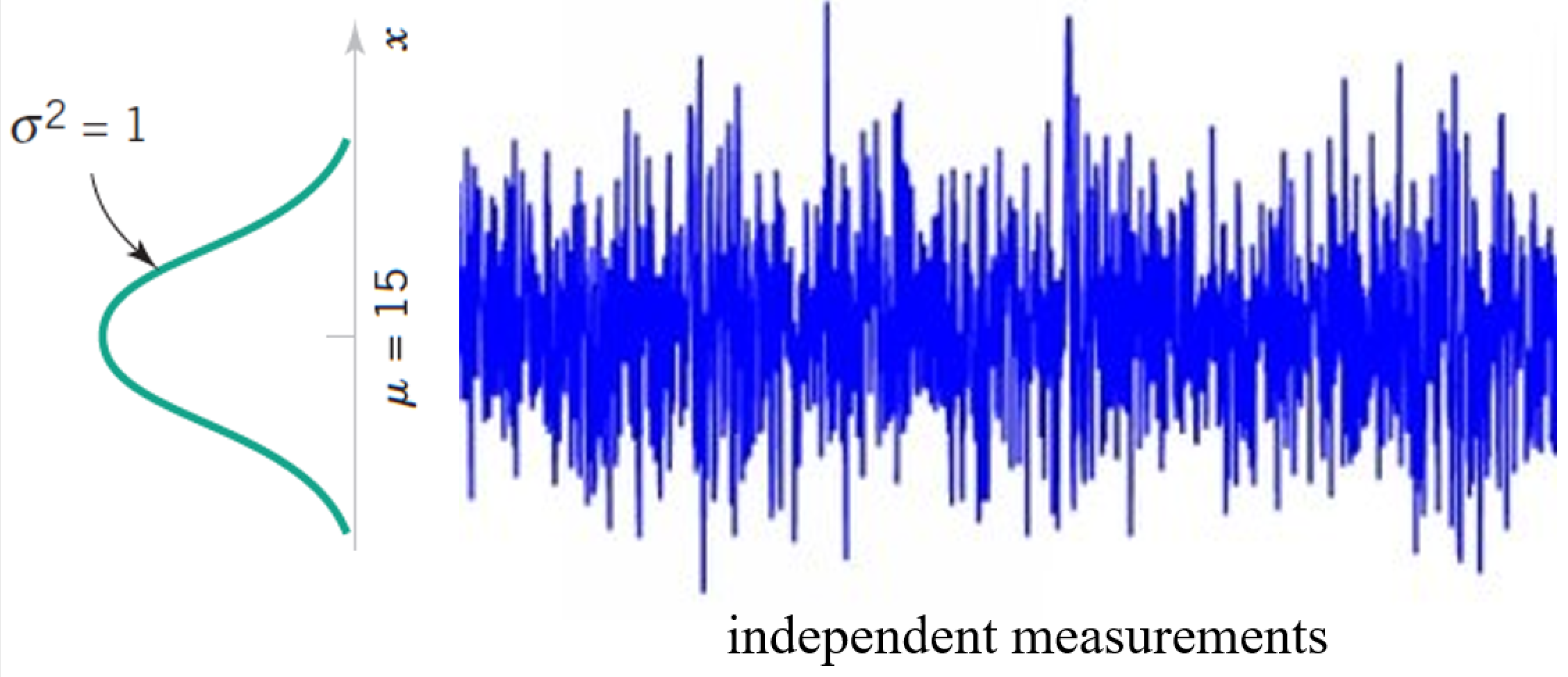
Now we say the noise is Normally distributed with zero-mean and variance $\sigma^2$. I.e. $\varepsilon_i \sim N(0,\sigma^2)$. The elements are independent and identically-distributed (i.i.d.).
What is the Likelihood $P(\mathbf y \,|\, \mathbf x)$?
Make a simpler optimization problem for finding the maximizer $\boldsymbol\beta^*$ for this scary thing.
Maximum a Posterior (MAP) Estimation
Again the system: $\mathbf y = \mathbf X \boldsymbol\beta + \boldsymbol\varepsilon$.
The noise is Normally distributed with $\boldsymbol\varepsilon \sim N(\mathbf 0,\sigma_2^2 \mathbf I)$.
Assume the solution has a prior $\boldsymbol\beta \sim N(\mathbf 0,\sigma_1^2 \mathbf I)$
Use Bayes Law to solve for the Posterior distribution.
Make a simpler optimization problem for finding the maximizer $\boldsymbol\beta^*$ for this monster.
Picture it
What does the prior do to our pictures?
Regression as Optimization
\begin{align} \text{Linear Regression: } \boldsymbol\beta_{lr}^* &= \arg\min\limits_{\boldsymbol\beta} \Vert \mathbf y - \mathbf X \boldsymbol\beta \Vert^2\\ \text{Ridge Regression: } \boldsymbol\beta_{rr}^* &= \arg\min\limits_{\boldsymbol\beta} \Vert \mathbf y - \mathbf X \boldsymbol\beta \Vert^2 + \lambda \Vert \boldsymbol\beta \Vert^2 \end{align}
Note these can be solved analytically with pseudoinverse or SVD techniques (which also provide some diffent kinds of variants).
...Analytical solutions...
Take home Messages
A quadratic residual minimization (e.g. norm-squared or variance) implies a Gaussian noise assumption.
A quadratic Penalty term implies a Gaussian prior assumption
The regularization parameter relates the variances of the noise and prior. Which we have to guess at (i.e. fit).
Maximum a Posterior (MAP) Estimation II
Again the system: $\mathbf y = \mathbf X \boldsymbol\beta + \boldsymbol\varepsilon$.
The noise is Normally distributed with $\boldsymbol\varepsilon \sim N(\mathbf 0,\sigma_2^2 \mathbf I)$.
Now the solution has a prior $\boldsymbol\beta \sim C \exp\big( \sum_i^n |\beta_i|\big)$. $C$ is a constant. This is sometimes called a Laplace distribution.
Use Bayes Law to solve for the Posterior distribution.
Make a simpler optimization problem for finding the maximizer $\boldsymbol\beta^*$ for this monster.
FYI: Full-on Bayesian Inference
While MAP estimation uses Bayes Law, it is not considered Bayesian inference typically.
Maximum Likelihood and MAP estimates are considered examples of "point estimates".
A Bayesian Inference technique estimates the entire posterior distribution, meaning $\boldsymbol\mu$ and $\boldsymbol\Sigma$ in the prior example.
We this we can estimate many things, such as,
- the mean value of $\boldsymbol\beta$ $\rightarrow$ a (better?) point estimate.
- the variance of $\boldsymbol\beta$ $\rightarrow$ confidence intervals.
Regression as Optimization (updated)
\begin{align} \text{Linear Regression: } \boldsymbol\beta_{lr}^* &= \arg\min\limits_{\boldsymbol\beta} \Vert \mathbf y - \mathbf X \boldsymbol\beta \Vert_2^2\\ \text{Ridge Regression: } \boldsymbol\beta_{rr}^* &= \arg\min\limits_{\boldsymbol\beta} \Vert \mathbf y - \mathbf X \boldsymbol\beta \Vert_2^2 + \lambda \Vert \boldsymbol\beta \Vert_2^2 \\ \text{"LASSO": } \boldsymbol\beta_{lasso}^* &= \arg\min\limits_{\boldsymbol\beta} \Vert \mathbf y - \mathbf X \boldsymbol\beta \Vert_2^2 + \lambda \Vert \boldsymbol\beta \Vert_1 \end{align}
Also Logistic version of everything for Classification.
Take home Messages (updated)
A $\ell_2$ residual minimization (e.g. norm-squared or variance) implies a Gaussian noise assumption.
A $\ell_2$ Penalty term implies a Gaussian prior assumption
A $\ell_1$ Penalty term implies a Laplace prior assumption
The regularization parameter relates the variances of the noise and prior. Which we have to guess at (i.e. fit).
Lab
Return to your regression lab.
Find $\ell_1$ and $\ell_2$ fits and compare.
Compute histograms of the residual and see how Gaussian it looks.
Estimate variance of residual. What does that suggest about the prior?
Formal Machine Learning Framework & Jargon 1/3
Given training data $(\mathbf x_{(i)},y_i)$ for $i=1,...,m$.
Choose a model $f(\cdot)$ where $f(\mathbf x)\approx y$
Define a loss function $L(f(\mathbf x), y)$ to minimize.
Formal Machine Learning Framework & Jargon 2/3
Have data $(\mathbf x_{(i)},y_i)$, model $f(\cdot)$, and loss function $L(f(\mathbf x), y)$.
Want to minimize true loss which is the expected value of the loss.
We approximate it by minimizing the Empirical loss (a.k.a "risk") $$ L_{emp}(f) = \frac{1}{m}\sum_{i=1}^m L\big(f(\mathbf x_{(i)}), y_i\big) $$ Emirical Risk minimization.
Formal Machine Learning Framework & Jargon 3/3
Emirical Risk minimization: $$ f^* = \arg \min\limits_f L_{emp}(f) = \arg \min\limits_f\frac{1}{m}\sum_{i=1}^m L\big(f(\mathbf x_{(i)}), y_i\big) $$ To trade-off model risk and simplicity, we include regularizer: $$ f^* = \arg \min\limits_f \big( L_{emp}(f) + \lambda R(f) \big) = \arg \min\limits_f L_{reg}(f) $$
Just cryptic talk for the same optimization problem we've been doing. But can be extended to cover many different techniques.
Machine Learning in bigger nutshell
Pick a model, e.g., $\mathbf y = \beta_0 + \beta_1 \mathbf x + \boldsymbol\varepsilon = f(\mathbf x;\beta_0, \beta_1) + \boldsymbol\varepsilon$ along with a risk function, e.g. $L = \Vert \mathbf y - f(\mathbf x;\beta_0, \beta_1) \Vert^2$ and a regularizer, e.g., $\Vert \boldsymbol \beta \Vert^2$.
"Fit" model to your data by using your favorite optimization technique to find parameters ($\beta^*_0, \beta^*_1$) that minimize Regularized Empirical Risk. $$ f^* = \arg \min\limits_f \Vert \mathbf y - f(\mathbf x;\beta_0, \beta_1) \Vert^2 + \lambda \Vert \boldsymbol \beta \Vert^2 $$
- Repeat #2 multiple times, adjusting hyperparameter $\lambda$ to trade-off model fit and complexity, checking performance using validation data.
Penalty Term Diversity
$\ell_1$
$\ell_2$
$\ell_{1,2}$. Mixed
Group
TV
Using Regression Methods for Classification
PLAN A: Directly apply regression. (How?)
PLAN B: Logistic regression.
NFL example:
- x axis is the number of touchdowns scored by team over a season
- y axis is whether they lost or won the game (0 or 1).
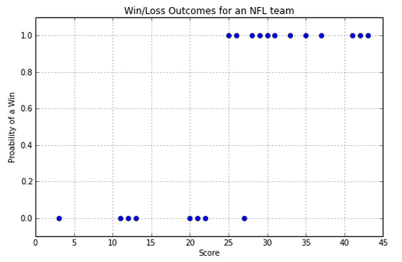
So, how do we predict whether we have a win or a loss if we are given a score? Note that we are going to be predicting values between 0 and 1. Close to 0 means we're sure it's in class 0, close to 1 means we're sure it's in class 1, and closer to 0.5 means we don't know.
Example - Linear Regression
Linear regression gets the general trend but it doesn't accurately represent the steplike behavior:
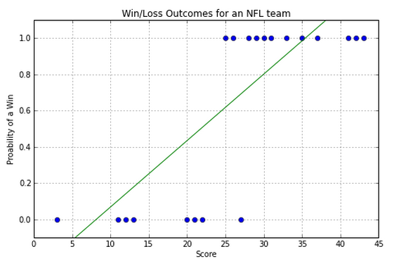
So a line is not the best way to model this data. Luckily we know of a better curve.
Logistic Regression - fit sigmoid curve instead of line
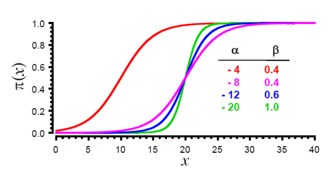
$$ f(x) = \frac{exp(\alpha+\beta x)}{1 + exp(\alpha+\beta x)} $$
Instead of choosing slope and intercept, choose parameters of sigmoid curve to fit the data.
Picture it: Classification versus Regression
one-dimensional case
two-dimensional case
Lab
Use scikit to perform classification using regression.
Try logistic, Ridge, and other regression methods.
Which are the most important features?
from sklearn.datasets import load_boston
boston = load_boston()
print(dir(boston))
print(boston.data.shape)
print(boston.feature_names)
print(boston.DESCR)