Outline
Bias versus Variance
Accuracy
Confusion Matrices
Related Metrics
ROC curves
import numpy as np
from matplotlib import pyplot as plt
%matplotlib inline
Formal Machine Learning Framework & Jargon 1/3
Given training data $(\mathbf x_{(i)},y_i)$ for $i=1,...,m$.
Choose a model $f(\cdot)$ where $f(\mathbf x)\approx y$
Define a loss function $L(f(\mathbf x), y)$ to minimize.
Formal Machine Learning Framework & Jargon 2/3
Have data $(\mathbf x_{(i)},y_i)$, model $f(\cdot)$, and loss function $L(f(\mathbf x), y)$.
Want to minimize true loss which is the expected value of the loss.
We approximate it by minimizing the Empirical loss (a.k.a "risk") $$ L_{emp}(f) = \frac{1}{m}\sum_{i=1}^m L\big(f(\mathbf x_{(i)}), y_i\big) $$ Emirical Risk minimization.
Formal Machine Learning Framework & Jargon 3/3
Emirical Risk minimization: $$ f^* = \arg \min\limits_f L_{emp}(f) = \arg \min\limits_f\frac{1}{m}\sum_{i=1}^m L\big(f(\mathbf x_{(i)}), y_i\big) $$ To trade-off model risk and simplicity, we include regularizer: $$ f^* = \arg \min\limits_f \big( L_{emp}(f) + \lambda R(f) \big) = \arg \min\limits_f L_{reg}(f) $$
Just cryptic talk for the same optimization problem we've been doing. But can be extended to cover many different techniques.
Machine Learning in bigger nutshell
Pick a model, e.g., $\mathbf y = \beta_0 + \beta_1 \mathbf x + \boldsymbol\varepsilon = f(\mathbf x;\beta_0, \beta_1) + \boldsymbol\varepsilon$ along with a risk function, e.g. $L = \Vert \mathbf y - f(\mathbf x;\beta_0, \beta_1) \Vert^2$ and a regularizer, e.g., $\Vert \boldsymbol \beta \Vert^2$.
"Fit" model to your data by using your favorite optimization technique to find parameters ($\beta^*_0, \beta^*_1$) that minimize Regularized Empirical Risk. $$ f^* = \arg \min\limits_f \Vert \mathbf y - f(\mathbf x;\beta_0, \beta_1) \Vert^2 + \lambda \Vert \boldsymbol \beta \Vert^2 $$
- Repeat #2 multiple times, adjusting hyperparameter $\lambda$ to trade-off model fit and complexity, checking performance using validation data.
Summary
Have data $(\mathbf x_{(i)},y_i)$, model $f(\cdot)$, and loss function $L(f(\mathbf x), y)$.
Regularized Emirical Risk minimization: $$ f^* = \arg \min\limits_f \big( L_{emp}(f) + \lambda R(f) \big) = \arg \min\limits_f L_{reg}(f) $$
Can be extended to cover classification techniques. (It's actually easier than regression)
Wait a minute..
Isn't it the job of the optimization algorithm to optimize the model?
Why are we evaluating the model? What can go wrong if we don't?
Bias in 100 words or less
Bias is when your assumptions about the true predictor affect the estimated predictor.
Example: you assume it is linear, use a linear model, get a linear result. If the true function is nonlinear, this linear model will have an error due to the bias.
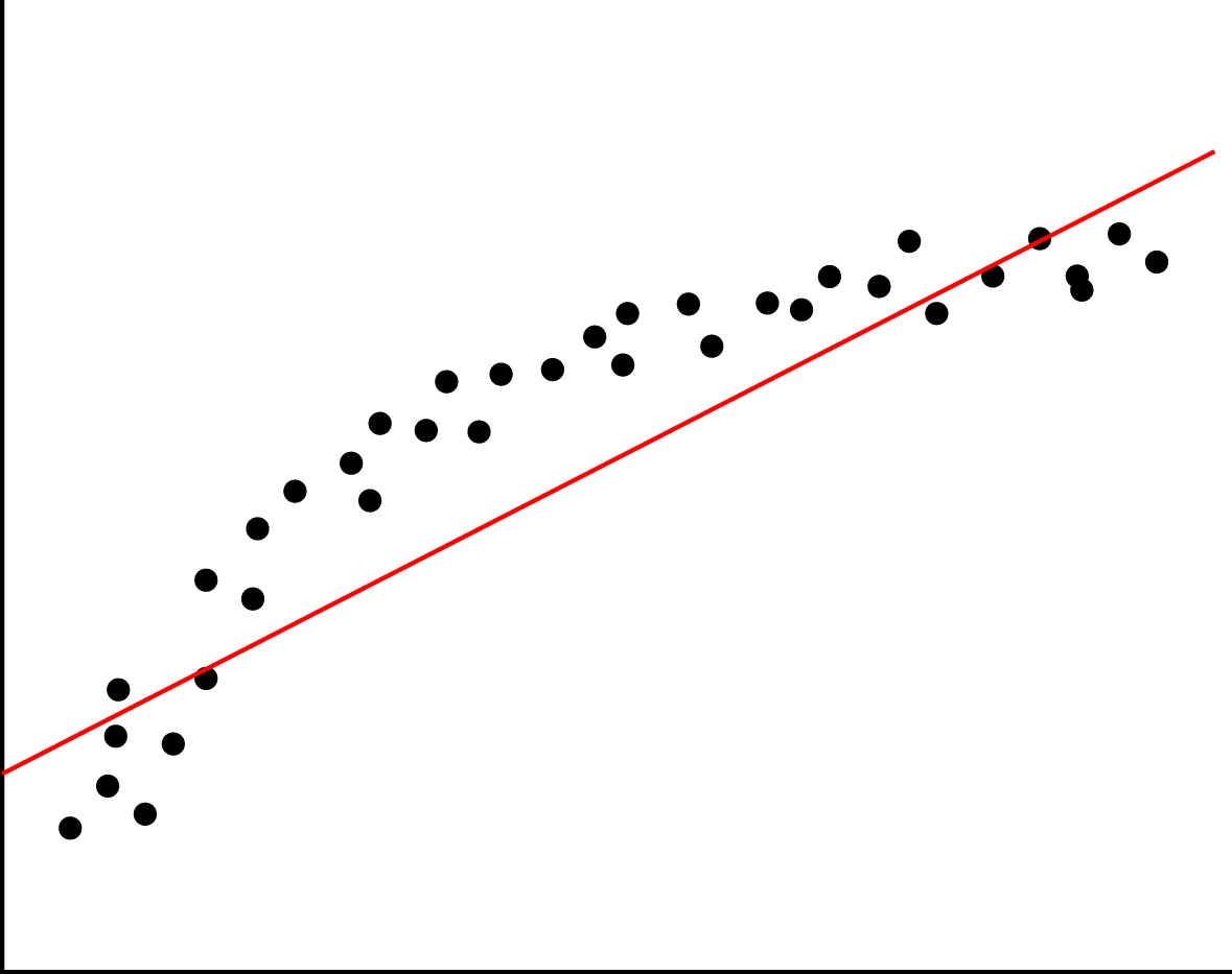
Formal definition: $$\text{Bias} = E(y - f(x))$$
Variance dumbed-down even further
Variance is when your model changes when fit using different sample.
I.e. it fits the noise $\varepsilon$ in addition to the true function
Out of fear of bias, we use a nonlinear model with way more parmeters to fit. It fits the (noisy) training data too well, and is worse than necessary on test data with different noise.
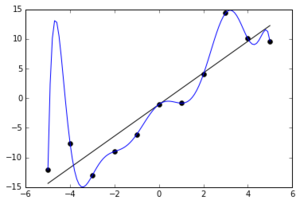
Formal definition: $$\text{Variance} = Var(f(x))$$
Bias-Variance Trade-off
Life is hard.
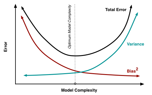
But then this is why Machine Learning experts make the big bucks.
Regularization as restriction on model complexity.
Lab
Generate Bias-Variance trade-off plot with larger example.
Validation
For choosing hyperparameters, best method
"Hold-out validation" ~ just test-train split.
Accepted/best approach depends on how much data you have:
Not enough: Cross Validation
Some: CV + Test set
Lots: Training set + Validation set + Test set
"Information leak" ~ test data affecting model
Other tips
Randomly shuffle data before splitting
If temporal sequence - make test set last (most future).
Classifier Metrics - Motivation
So why do we need classifier metrics? (name two reasons?)
Would the same metric work for both reasons?
Review
A classification problem is when we're trying to predict a discrete (categorical) outcome. We'll start with binary classification (i.e., yes/no questions).
Here are some example questions:
- Does a patient have cancer?
- Will a team win the next game?
- Will the customer buy my product?
- Will I get the loan?
In binary classification, we (often) assign labels of 0 and 1 to our data.
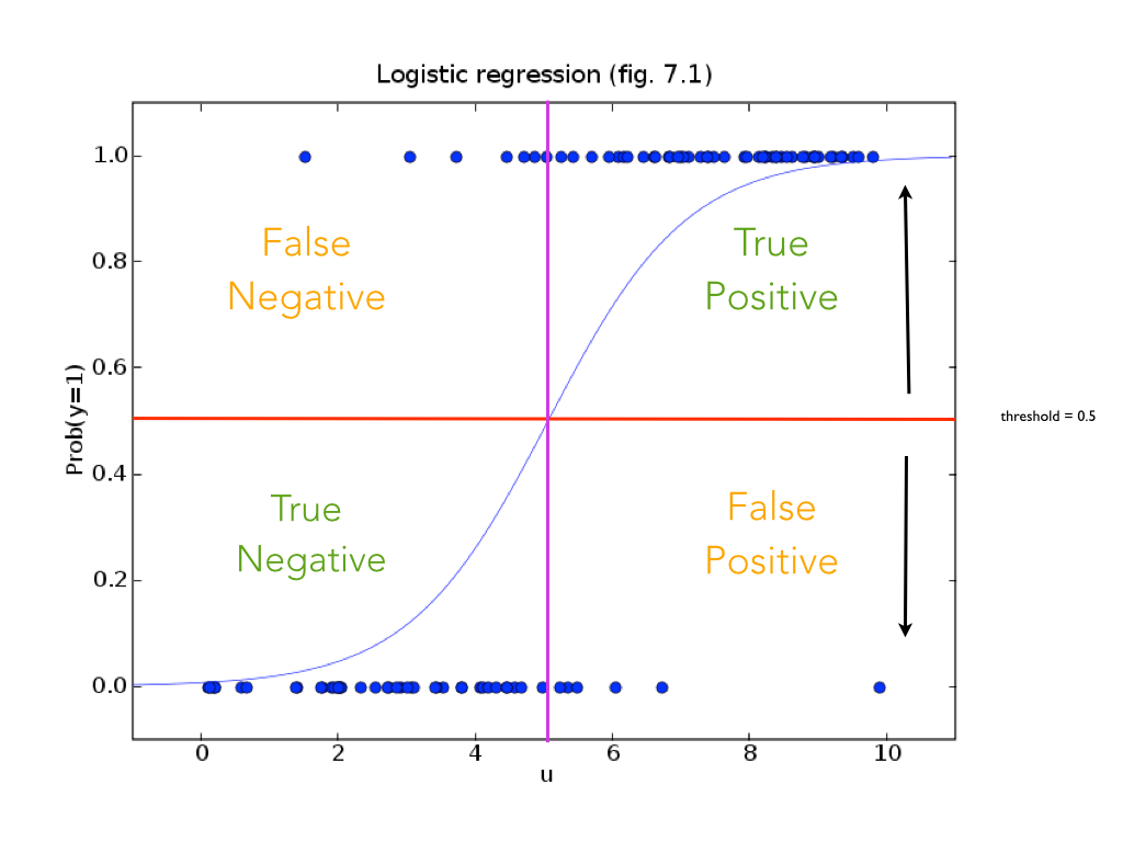
NFL example:
- x axis is the number of touchdowns scored by team over a season
- y axis is whether they lost or won the game (0 or 1).
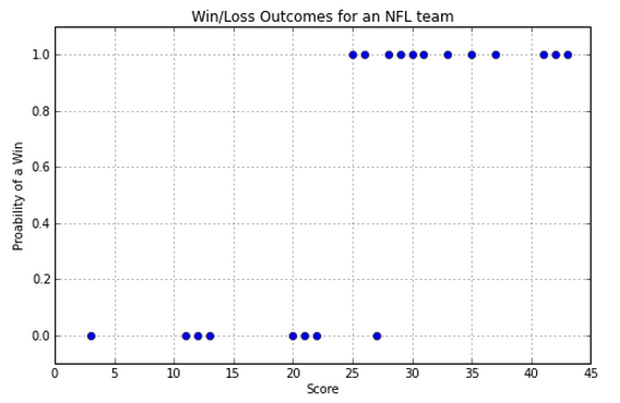
So, how do we predict whether we have a win or a loss if we are given a score? Note that we are going to be predicting values between 0 and 1. Close to 0 means we're sure it's in class 0, close to 1 means we're sure it's in class 1, and closer to 0.5 means we don't know.
Consider what linear regression, Logistic regression, and binary classification do here.
Accuracy
The simplest measure is accuracy. This is the number of correct predictions over the total number of predictions. It's the percent you predicted correctly. In sklearn, this is what the score method calculates.
Shortcomings
Accuracy is a good first glance measure, but it has shortcomings.
If the classes are unbalanced, accuracy will not measure how well you did at predicting. Say you are trying to predict whether or not an email is spam. Only 2% of emails are in fact spam emails. You could get 98% accuracy by always predicting not spam. This is a great accuracy but a horrible model!
What additional measurements might we do to check for such failures?
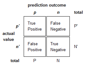
Confusion Matrix
We can get a better picture our model by looking at the confusion matrix. We get the following four metrics:
- True Positives (TP): Correct positive predictions
- False Positives (FP): Incorrect positive predictions (false alarm)
- True Negatives (TN): Correct negative predictions
- False Negatives (FN): Incorrect negative predictions (a miss)
Other popular scores: Precision, Sensitivity and F1
- Precision: A measure of how good your positive predictions are
Precison = TP / (TP + FP) = TP / (predicted yes) = fraction of correct 1's - Sensitivity: A measure of how well you predict positive cases. Aka recall.
Sensitivity = TP / (TP + FN) = TP / (actual yes) - F1 Score: The harmonic mean of Precision and Sensitivity
  F1 = 2 / (1/Precision + 1/Sensitivity)
     = 2 * Precision * Recall / (Precision + Sensitivity)
     = 2TP / (2TP + FN + FP)
Youden Index
Youden's Index (sometimes called J statistic) is similar to the F1 score in that it is a single number that describes the performance of a classifier.
$$J = Sensitivity + Specificity - 1$$
$$where$$
$$Sensitivity = \frac{TP}{TP + FN}$$
$$Specificity = \frac{TN}{TN + FP}$$
The J statistic ranges from 0 to 1:
- 0 indicating that the classifier does no better than random
- 1 indicating that the test performed perfectly
It can be thought of as an improvement on the F1 score since it takes into account all of the cells in a confusion matrix. It can also be used to find the optimal threshold for a given ROC curve.
Quiz
- What tools do you have at your disposal to change TP, FP, TN and FN?
- Some of you used linear regression to predict the 2-4 labels on the breast cancer data set. What could you do with the output from that model to get your classifier to correctly classify every positive exaple?
- In what ways would performance suffer?
Exercise 1. Calculating confusion matrix quantities
Suppose that you're using linear regression to predict 0-1 labels. You train your model and on the test data you get the following results. Calculate TP, FP, TN, FN
labels = [0,0,0,0,0,1,1,1,1,1]
predictions = [-0.8, -0.4, 0.0, 0.4, 0.8, 0.2, 0.6, 1.0, 1.4, 1.8]
threshold = .5

#calculate TP, FP, TN, FN
Example 2. Suppose some mistakes are more expensive than others
Now suppose
- the cost of a false positive is 1
- the cost of a false negative is 10
- true positive and false positive cost zero.
How much does your predictor cost with a threshold value of 0.5?
Generate costs for threshold values of 0.0, 0.25, 0.5, 0.75 and 1.0.
Which one yields the minimum cost?
Explain any shift in the threshold from 0.5.
ROC Curves
Very popular way to visualize classifier performance. (http://en.wikipedia.org/wiki/Receiver_operating_characteristic)
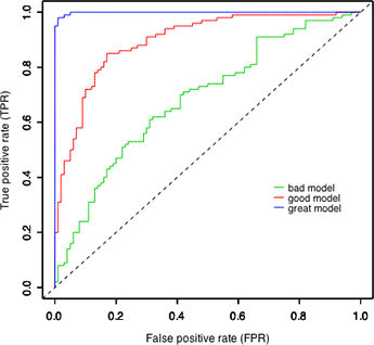
ROC curve = true positive rate (TPR) versus false positive rate (FPR).
\begin{align} \text{True Positive Rate} &= TPR = \frac{\text{number of true positives}}{\text{number of actual positives}} \\ \text{False Positive Rate} &= FPR = \frac{\text{number of false positives}}{\text{number of actual negatives}} \\ \end{align}
ROC Curves
\begin{align} \text{True Positive Rate} &= TPR = \frac{\text{number of true positives}}{\text{number of actual positives}} \\ \text{False Positive Rate} &= FPR = \frac{\text{number of false positives}}{\text{number of actual negatives}} \\ \end{align}
What are the rates for random guessing?
Example 3.
- Write an ROC curve function to compute several points on the ROC curve for the toy problem above. Then plot the result (TPR versus FPR).
- What happens if you choose a threshold value and generate hard 0-1 labels before calculating the ROC curve?
import numpy as np
import matplotlib.pyplot as plt
%matplotlib inline

labels = [0,0,0,0,0,1,1,1,1,1]
predictions = [-0.8, -0.4, 0.0, 0.4, 0.8, 0.2, 0.6, 1.0, 1.4, 1.8]
Thought Lab
When you use KNN as your prediction algorithm you have two choices on this binary classification problem. You can use regression version of KNN or classification version of KNN.
- What happens if you take as output from kNN classifier, the majority class? What your alternative?
- What is the difference in the way the labels are calculated?
- What is the difference in the ROC curve?
Lab Exercise 2.
- Plot a ROC curve for the breast cancer data using whatever predictions are handy for you.
# import pandas as pd
import numpy as np

with open('breast-cancer-wisconsin.data.txt') as f:
    data = f.readlines()

cleaned_list= []
for x in data:
    if "?" not in x:
        cleaned_list.append(x)

list_of_lists = []
for x in cleaned_list:
    temp = x.replace("\n", "").split(",")
    row = [float(z) for z in temp]
    list_of_lists.append(row)

list_of_lists = np.array(list_of_lists)
list_of_lists.shape
list_of_lists[:,1:].shape

no_ids = list_of_lists[:,1:]
X = no_ids[:,:-1]
y = no_ids[:,-1]  # labels
# x.shape
# y.shape
Feature Engineering & Feature Selection
Pick only features most correlated with target
Use L1 regression and use features with nonzero coefficient $\beta$
Use domain knowledge to intelligently compute better features (heuristic)
- symmetries, transforms, filters
Be careful of information leaks!
Preprocessing
Normalization / standardization
Vectorizing missing values
Convert text to numbers
Dealing with missing values
Information leak danger