Outline
- Primal SVM
- Dual SVM
- Kernels and Nonlinear Models (for everyone)
import numpy as np
from matplotlib import pyplot as plt
%matplotlib inline
Recall: Optimization for Regression
A framework for describing problems for minimizing/maximizing functions Plus an "art" for finding easier alternative problems that have same minimizer.
\begin{align} \text{minimizer: } \boldsymbol\beta^* &= \arg\min\limits_{\boldsymbol\beta} g(\boldsymbol\beta) \\ \text{minimum: } g_{min} &= \min\limits_{\boldsymbol\beta} g(\boldsymbol\beta) = g(\boldsymbol\beta^*) \end{align}
Linear system: $\mathbf y = \mathbf X \boldsymbol\beta + \boldsymbol\varepsilon$.
What is "$g$" and $\mathbf z$
What is the differnce between the minimizer and the minimum?
Draw the residual we are minimizing on a 1D regression, and 1D classification.
Recall: Regression for Classification
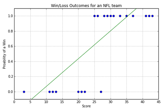
All we really want is the best cutoff between the two classes.
How would we mathematically write the residual for that?
Multidimensional Case
Write out multidimensional version for a collection of labeled data we wish to classify correctly.
Bonus: Combine into a matrix expression.
Constrained Optimization
Easy problems: \begin{align} \boldsymbol\beta^* &= \arg\min\limits_{\boldsymbol\beta} g(\boldsymbol\beta) \\ \end{align}
Where the action is: \begin{align} \begin{array}{c} \boldsymbol\beta^* = \\ \; \\ \; \end{array} \begin{array}{c} \arg\min\limits_{\boldsymbol\beta} g(\boldsymbol\beta) \\ \mathbf V \boldsymbol\beta = \mathbf z \\ \mathbf W \boldsymbol\beta \ge \mathbf w \end{array} \end{align}
The added equation and inequality are called constraints.
Convex Optimization
Linear Program: \begin{align} \begin{array}{c} \boldsymbol\beta^* = \\ \; \\ \; \end{array} \begin{array}{c} \arg\min\limits_{\boldsymbol\beta} \mathbf c^T \boldsymbol\beta \\ \mathbf V \boldsymbol\beta = \mathbf z \\ \mathbf W \boldsymbol\beta \ge \mathbf w \end{array} \end{align}
Quadratic Program: \begin{align} \begin{array}{c} \boldsymbol\beta^* = \\ \; \\ \; \end{array} \begin{array}{c} \arg\min\limits_{\boldsymbol\beta} \boldsymbol\beta^T \mathbf H \boldsymbol\beta \\ \mathbf V \boldsymbol\beta = \mathbf z \\ \mathbf W \boldsymbol\beta \ge \mathbf u \end{array} \end{align}
Semidefinite Program...
Geometric Program...
The Optimization Game:
make your optimization problem into one of these using linear algebra and other tricks.
Use off-the-shelf solver to optimize it for you
So how might we fit a classification in?
Lab - using optimization to do classification
Try different objectives to deal with multiple solutions
Think of ways to deal with non-separable data
Maximizing the margin
Suppose we try to maximize the margin for each term?
Just draw what this does for each term.
Primal SVM
Show that with a couple more tricks we can achieve same thing with the following:
Suport-Vector Machine ("primal form"): \begin{align} \begin{array}{c} \boldsymbol\beta^* = \\ \; \end{array} \begin{array}{c} \arg\min\limits_{\boldsymbol\beta} \boldsymbol\beta^T\boldsymbol\beta \\ y_{(i)} \left(\mathbf x_{(i)}^T\boldsymbol\beta + b \right) \ge 1, \; i=1,...,m \end{array} \end{align}
where the training data is $\left(\mathbf x_{(i)}, y_{(i)} \right), , \; i=1,...,m$.
Soft Margin
\begin{align} \begin{array}{c} \boldsymbol\beta^* = \\ \; \end{array} \begin{array}{c} \arg\min\limits_{\boldsymbol\beta} \frac{1}{m}\sum_i \delta_i + \mu \boldsymbol\beta^T\boldsymbol\beta \\ y_{(i)} \left(\mathbf x_{(i)}^T\boldsymbol\beta + b \right) \ge 1 - \delta_i, \; i=1,...,m \end{array} \end{align}
Maximum margins implies Support vectors
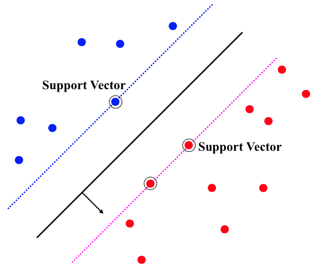
Dual SVM
With convex optimization theory, one can make an equivalent problem that utilizes support vectors instead of samples
\begin{align} \begin{array}{c} \boldsymbol\beta^* = \\ \; \end{array} \begin{array}{c} \arg\min\limits_{\mathbf c} \sum_i c_i - \frac{1}{2} \sum_i \sum_j y_i c_i \mathbf x_i^T \mathbf x_j y_j c_j \\ \sum_i c_i y_i = 0, 0 \le c_i \le \frac{1}{2n\mu}, \; i=1,...,m \end{array} \end{align}
Looks scary, but the important fact is it only uses terms like $\mathbf x_i^T \mathbf x_j$, never $\mathbf x_i$ alone.
Lab
Using scikit, implement linear SVM.
Then try implementing a nonlinearity that can separate data radially, by manually transforming the data.
Try built-in kernels on the data instead.
Nonlinear Decision Boundaries
Any classifier can be extended to make a nonlinear decision boundary by augmenting or replacing samples $\mathbf x_i$ with samples $f(\mathbf x_i)$, where $f(\cdot)$ is a nonlinear function we choose.
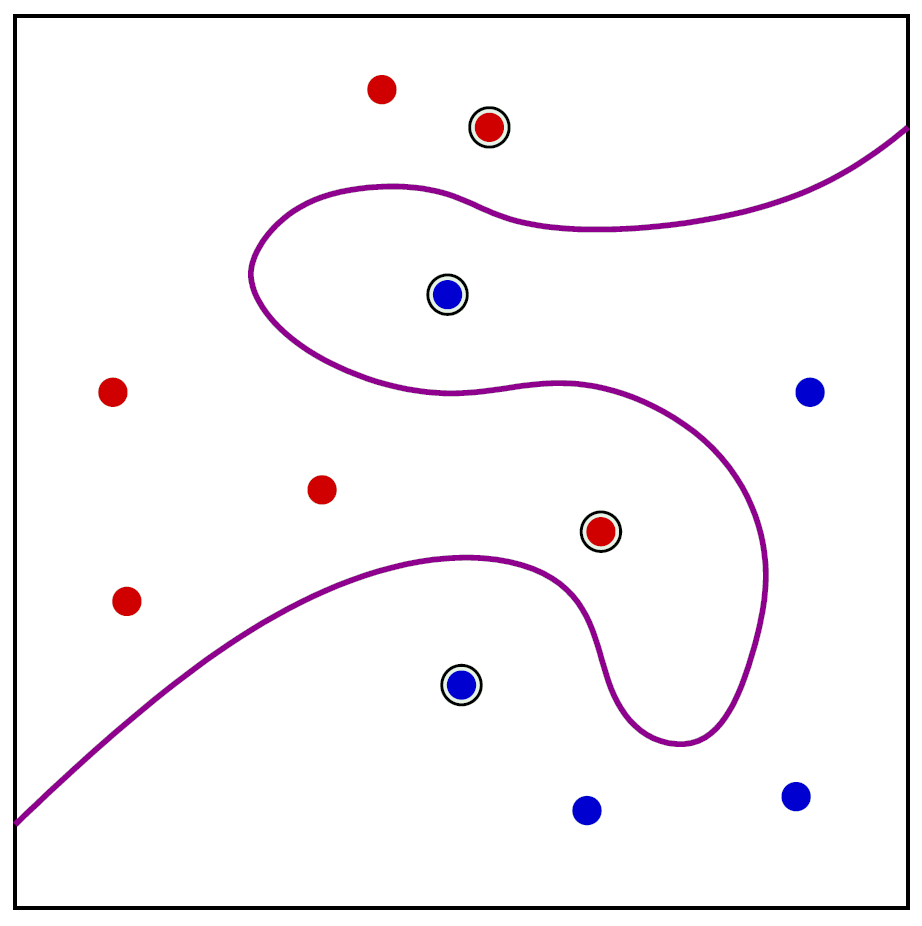
Not as amazing as it may seem, since we have to know the shape we want. Basically we warp the coordinate system and do a linear classifier in the new warped space.
Basis functions
Recall the training data is $\left(\mathbf x_{(i)}, y_{(i)} \right), , \; i=1,...,m$.
And the application to new unknown data will be some $\mathbf x'$ where we seek to determine $y'$
A "Basis Function Expansion" replaces $\mathbf x$ with some new vector $\mathbf z$ where each element is a different function of the elements of $\mathbf x$.
$$ \mathbf z = \boldsymbol\phi(\mathbf x) = \begin{pmatrix}\phi_1(\mathbf x) \\ \phi_2(\mathbf x) \\ \vdots \\ \phi_p(\mathbf x) \end{pmatrix} $$
Ex: convert cartesian to polar coordinates.
Dual SVM tricks
Since SVM's can be made to operate only on inner products of samples using dual version (i.e., $\mathbf x_i^T \mathbf x_j$).
What happens when we transform coordinates to some nonlinear basis?
Kernels
$\boldsymbol\phi(\mathbf x_i)^T \boldsymbol\phi(\mathbf x_j) = K(\mathbf x_i, \mathbf x_j)$
It can be very easy to compute $(\mathbf x_i, \mathbf x_j)$ though it is very difficult to compute $\boldsymbol\phi(\mathbf x_i)$ and $\boldsymbol\phi(\mathbf x_j)$ (it may even be impossible to compute them).
Many find this very exciting.
Popular kernels available in software packages benefit from this trick.
Radial Basis Function (RBF) Kernel
$$ K(\mathbf x_i, \mathbf x_j) = \exp\left(-\frac{1}{2\sigma^2} \Vert \mathbf x_i - \mathbf x_j \Vert^2 \right) $$
Most popular one probably.