Outline
- Homeworks 5 & 6
- Regression for Classification
- Activation functions
- Multilayer Perceptron and tensors
import numpy as np
from matplotlib import pyplot as plt
%matplotlib inline
Recall Regression $\mathbf y = f(\mathbf x;\beta_0, \boldsymbol\beta) + \boldsymbol\varepsilon $
Simple Linear Regression, $f(\mathbf x;\beta_0, \boldsymbol\beta) = \beta_0 + \boldsymbol\beta x$
Minimize $e^2 = \Vert \mathbf y - f(\mathbf x;\beta_0, \boldsymbol\beta) \Vert^2$ to find optimal $\boldsymbol\beta$ ~ LMS Loss
- Plan A. Guesstimate $\beta_0$, $\boldsymbol\beta$ by eye
- Plan B: analytically find minimizer using calculus
- Plan C: Use optimization - Newton method, LARS, gradient descent...
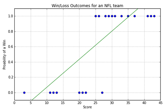
Regression for Classification
- Simple Linear Regression, $f(\mathbf x;\beta_0, \boldsymbol\beta) = \beta_0 + \boldsymbol\beta^T \mathbf x$
Minimize $e^2 = \Vert \mathbf y - f(\mathbf x;\beta_0, \boldsymbol\beta) \Vert^2$ to find optimal $\boldsymbol\beta$ ~ LMS Loss, ak.a L2, Least Squares
- Logistic Regression $f(\mathbf x;\beta_0, \boldsymbol\beta) = sigmoid(\beta_0 + \boldsymbol\beta^T \mathbf x)$
$$sigmoid(z) = \frac{1}{1+e^{-z}}$$
How might we fit this one?
Derivative of Sigmoid
$$ \frac{\partial}{\partial z} sigmoid(z) = \frac{\partial}{\partial z} \frac{1}{1+e^{-z}} = ... ? $$
$$ \frac{\partial}{\partial z} sigmoid(z) = sigmoid(z) (1 - sigmoid(z)) $$
Setting this equal to zero doesn't work, but with enough time and computing resources you can minimize anything, especially if you can compute the gradient...
Gradient Descent
Went from too-trivial-to-cover in optimization classes, to the current state-of-the-art due to massive data sizes and parallel computing
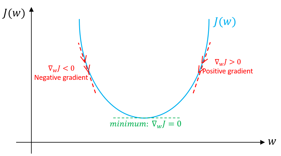
Apply this to a toy problem.
What do we use for the step size?
Matrix Calculus
https://en.wikipedia.org/wiki/Matrix_calculus
https://www.math.uwaterloo.ca/~hwolkowi/matrixcookbook.pdf
"The Matrix Calculus You Need For Deep Learning" https://arxiv.org/abs/1802.01528
"This paper is an attempt to explain all the matrix calculus you need in order to understand the training of deep neural networks. We assume no math knowledge beyond what you learned in calculus 1...
Gradient Descent - improvements (or sometimes not...)
Stochastic
Acceleration
Adaptive step sizes
Averaging of steps
...
Stochastic Gradient Descent
Considered one of the key reasons for Deep Learning's success
Conventional gradient descent uses entire dataset to compute step.
Stochastic gradient descent uses randomly-chosen sample to make steps.
Batch stochastic gradient descent uses small batches to compute a step.
Epoch = single pass through the entire dataset in batch steps.
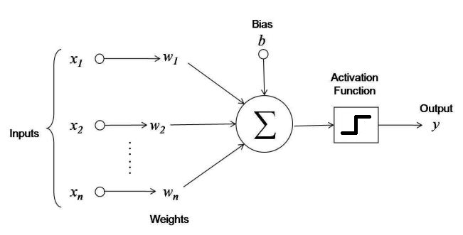
The Perceptron
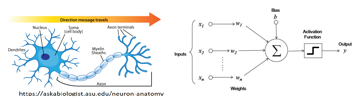
\begin{align} f(\mathbf x) = f(x_1, x_2, ..., x_n) &= \begin{cases} +1, \text{ if } \sum_{i=1}^{n}w_i x_i + b > 0 \\ -1, \text{ if } \sum_{i=1}^{n}w_i x_i + b < 0 \end{cases} \\ &= \text{sign}\left\{ \sum_{i=1}^{n}w_i x_i + b \right\} = \text{sign}(\mathbf w^T \mathbf x) \end{align}
"Fire or not-fire" decision.
Look familiar??
Perceptron Learning Algorithm
choose starting $\mathbf w$, $b$, stepsize $\eta$.
For each $(\mathbf x_i, y_i)$: test $f(\mathbf w,b, \mathbf x_i) = y_i$?
- If $f(\mathbf w,b, \mathbf x_i) \neq y_i$, set $(\mathbf w,b) = (\mathbf w,b) + \eta \, y_i \times (\mathbf x_i,1)$
Can view this algorithm as gradient descent for the loss function:
$$ L(f(\mathbf x_i), y_i) = \max(0, -y_i \mathbf w^T (\mathbf x_i,1)) $$
N = 100
X = np.random.rand(N,2)*100000

w_true = np.array([2,-1])
b_true = -30000
f_true = lambda x :np.sign(w_true[0]*x[0]+w_true[1]*x[1] + b_true);

y = np.zeros([N,1])
for i in np.arange(0,len(X)):
    x_i = X[i]
    y_i = f_true(x_i)
    y[i] = y_i
    #print(i,x_i,y_i)
    if y_i==-1: # negative samples
        plt.scatter(x_i[0], x_i[1], s=120, marker='_', linewidths=2,color='r')
    if y_i==1: # positive samples
        plt.scatter(x_i[0], x_i[1], s=120, marker='+', linewidths=2,color='b')
plt.xlabel('income');
plt.ylabel('debt');
plt.plot([(-b_true-100000*w_true[1])/w_true[0],-b_true/w_true[0]],[100000,0]); # example hyperplane

w = np.zeros(2)
b = np.zeros(1)
f = lambda w,b,x :np.sign(w[0]*x[0]+w[1]*x[1] + b);

acc = np.zeros([N,1])

print(w)
eta = 1e-5;
for i in np.arange(0,len(X)):
    x_i = X[i]
    y_i = y[i]
    print(x_i, y_i, f(w,b,x_i), w,b)
    for j in np.arange(0,len(X)):
      acc[i] = acc[i] + y[j]*f(w,b,X[j])/len(X);
    if(y_i != f(w,b,x_i)): # If not classified correctly, adjust the line to account for that point.
       b = b + 1e5*eta*y_i;
       w[0] = w[0] + eta*y_i*x_i[0];
       w[1] = w[1] + eta*y_i*x_i[1];


for i in np.arange(0,len(X)):
    x_i = X[i]
    y_i = f_true(x_i)
    if y_i==-1: # negative samples
        plt.scatter(x_i[0], x_i[1], s=120, marker='_', linewidths=2,color='r')
    if y_i==1: # positive samples
        plt.scatter(x_i[0], x_i[1], s=120, marker='+', linewidths=2,color='b')
plt.xlabel('income');
plt.ylabel('debt');

plt.plot([(-b_true-100000*w_true[1])/w_true[0],-b_true/w_true[0]],[100000,0]); # true hyperplane

plt.plot([(-b-100000*w[1])/w[0],-b/w[0]],[100000,0]); # estimated hyperplane

plt.figure();
plt.plot(acc); # estimated accuracy
plt.xlabel('iteration');
plt.ylabel('accuracy');


Activation Functions
Key nonlinearity needed for Artificial Neural Networks to do anything interesting.
Consider what happens with networks of ANN's with no activation function.
Note these are scalar functions with scalar inputs. First compute the inner product then apply function.
Activation Functions - Step function
First big idea, from 1950's.
Essentially same as sign function.
$$ f(\mathbf x) = \text{sign}(\mathbf w^T \mathbf x) $$
No good way to train big networks made of these, so this function isn't used.
x = np.arange(-10, 10, 0.1)
plt.plot(x, np.sign(x), linewidth=3);
plt.xlabel('x');
plt.ylabel('sign(x)');

Activation Functions - Sigmoid
$$\sigma(x) = \frac{1}{1 + e^{-x}}$$
The next popular option that came along, can optimize by taking gradients because smooth.
x = np.arange(-10, 10, 0.1)
plt.plot(x, 1 / (1 + np.exp(-x)), linewidth=3);
plt.xlabel('x');
plt.ylabel('sigma(x)');

Activation Functions - Rectified Linear Unit "ReLU"
$$ \text{ReLU}(x) = \alpha \max(0,x)= \begin{cases} 0, \text{ if } x < 0 \\ \alpha x, \text{ if } x > 0 \end{cases} $$
The activation function that was popular when Deep Learning became famous.
Not smooth but gradient still simple to do computationally.
Variants such as "Leaky ReLU" improve implementation details.
x = np.arange(-10, 10, 0.1)
plt.plot(x, [max(0, i) for i in x], linewidth=3);
plt.xlabel('x');
plt.ylabel('ReLU(x)');

Multilayer (Artificial) Neural Networks - "Feed forward"
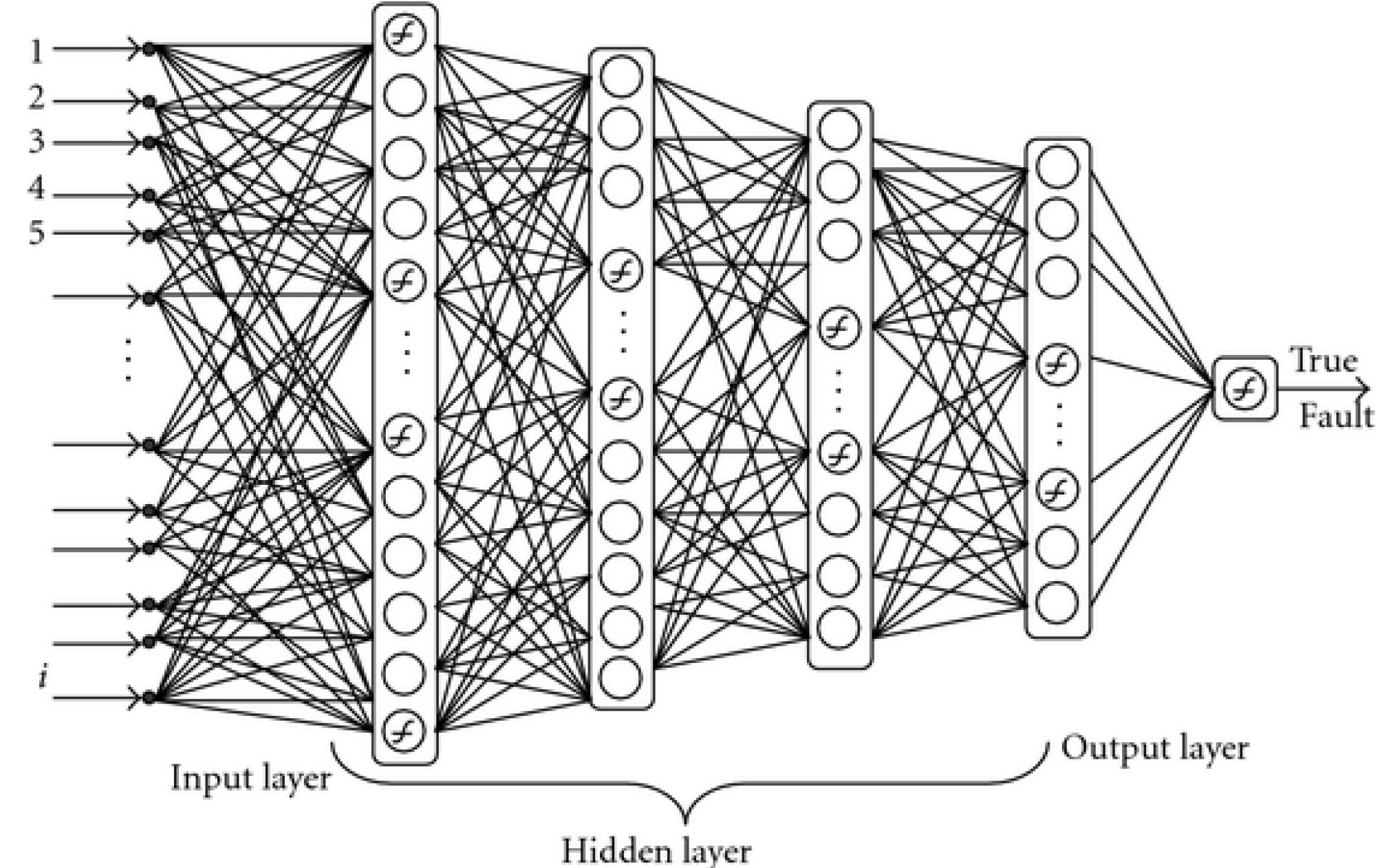
How do we even decide what neurons to connect where and all?
Tensor Perspective
Input data $\mathbf x$ can be viewed as vectors, matrices, or beyond... generally called "tensors"
Consider a layer with multiple outputs (e.g. multi-class classifier) $$ f_1(\mathbf x) = \hat{y}_1 \\ f_2(\mathbf x) = \hat{y}_2 \\ ... $$ Layers themselves viewed as functions on tensors.
$$ "\mathbf f(\mathbf x)" = \hat{\mathbf y} $$
Multiple Layers in Tensor perspective
Two-layer network as concatenated single-layer networks: $$ \mathbf f^{(1)}(\mathbf x) = \hat{\mathbf y}^{(1)} \\ \mathbf f^{(2)}(\mathbf x) = \hat{\mathbf y}^{(2)} \\ ... $$ Multilayer network as composition of tensor functions $$ \mathbf f^{(2)}\big(\mathbf f^{(1)}(\mathbf x) \big) = \hat{\mathbf y}^{(2)} \\ $$
Just another model to fit: $$ f_{(entire\_network)}(\mathbf x) = \hat{y} $$
Need to take care that input and output sizes match
Optimize a big Loss function of everything
Optimize Neural Nets
As always, we want to minimize a loss function: $L(f(\mathbf x),y)$.
Current state-of-the-art:
- Many loss functions possible (next class)
- Regularization (can change per-layer), L1, L2, Dropout, "early stopping"
- Minimize using gradient descent (Backpropagation algorithm -- next semester).
Regularization
L2 (a.k.a. weight decay) implies we do what?
L1?
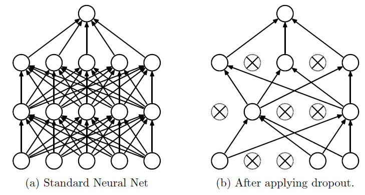
Dropout...
Dropout
Deep Architecture
AlexNet:
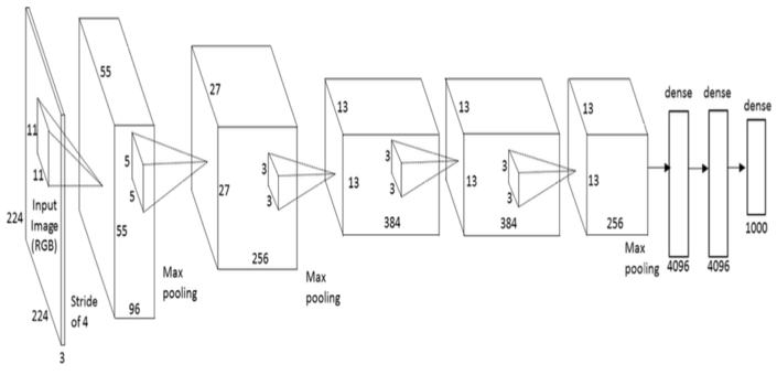
"Imagenet classification with deep convolutional neural networks" A Krizhevsky, I Sutskever, GE Hinton, NIPS 2012
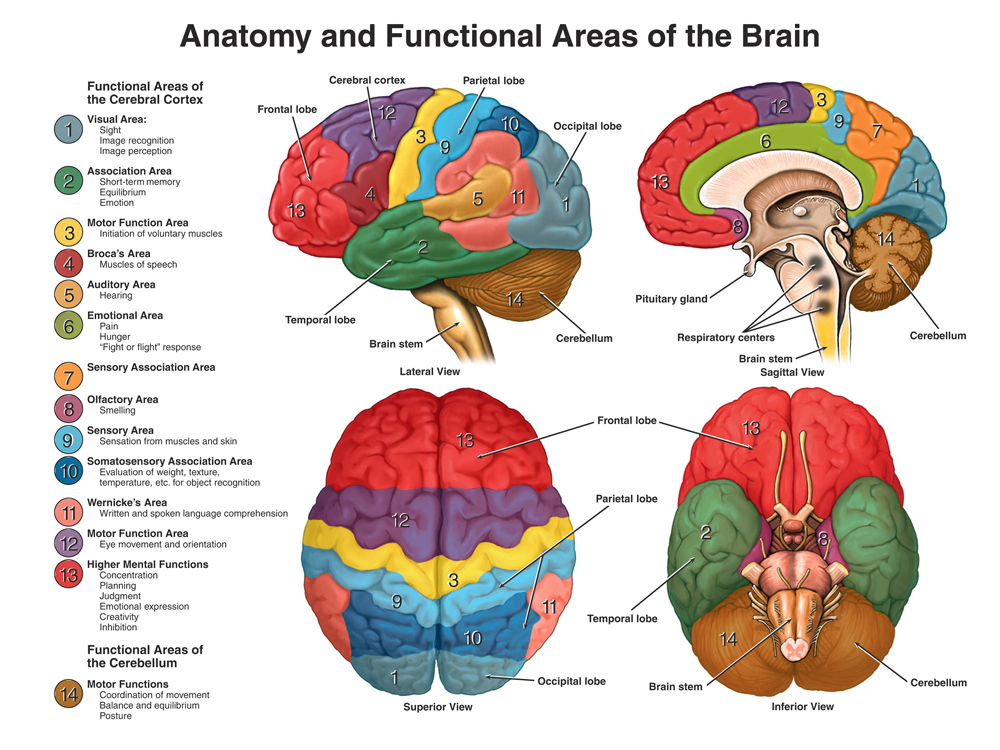
Basically we try stuff using intuition and (educated?) guesswork. Special kinds of layers, based on biological inspiration from the vision system, are very popular due to sucesses in Machine Learning competitions.
Lab: Install Tensorflow & Keras
Ideally using Anaconda.
Or via command line:
conda create -n tensorflow_py36 python=3.6
conda activate tensorflow_py36
conda install tensorflow
conda install keras
conda install matplotlib numpy (and whatever else...)
Or from within Anaconda-Navigator using GUI.
Plan B: Cloud-based Notebooks
Google CoLab: https://colab.research.google.com/notebooks/welcome.ipynb
Kaggle Kernel: https://www.kaggle.com/kernels