Outline
- Keras API
- CNN example
import numpy as np
from matplotlib import pyplot as plt
%matplotlib inline
Install Tensorflow & Keras
Ideally using Anaconda.
Command line:
conda create -n tensorflow_py36 python=3.6
conda activate tensorflow_py36
conda install tensorflow
conda install keras
conda install matplotlib (and whatever else...)
Or from within Anaconda-Navigator using GUI.
Plan B: Cloud-based Notebooks
Google CoLab: https://colab.research.google.com/notebooks/welcome.ipynb
Kaggle Kernel: https://www.kaggle.com/kernels

Chollet Book (Google employee who worked on Keras)
Tries to be very practical, non-mathematical (uses code to explain concepts).

Formal Machine Learning Framework & Jargon 1/3
Given training data $(\mathbf x_{(i)},y_i)$ for $i=1,...,m$.
Choose a model $f(\cdot)$ where $f(\mathbf x)\approx y$
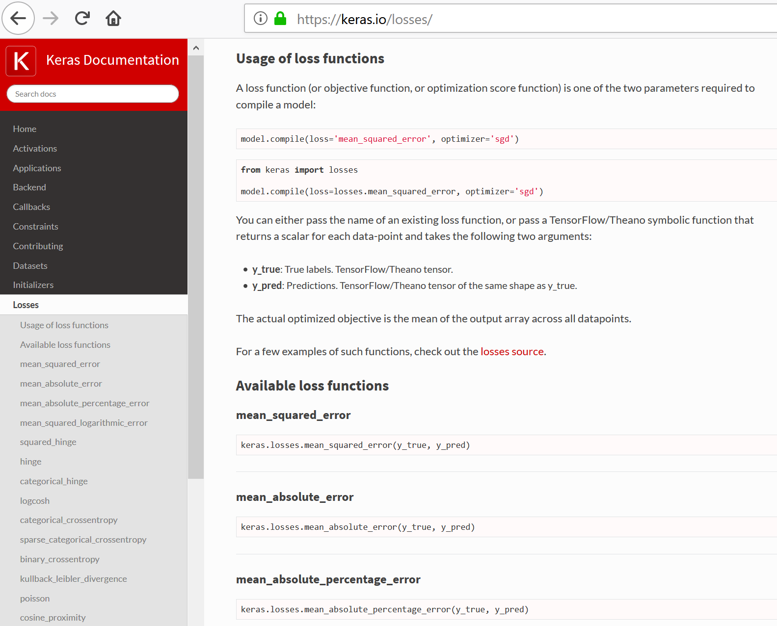
Define a loss function $L(f(\mathbf x), y)$ to minimize.
Formal Machine Learning Framework & Jargon 2/3
Have data $(\mathbf x_{(i)},y_i)$, model $f(\cdot)$, and loss function $L(f(\mathbf x), y)$.
Want to minimize true loss which is the expected value of the loss.
We approximate it by minimizing the Empirical loss (a.k.a "risk") $$ L_{emp}(f) = \frac{1}{m}\sum_{i=1}^m L\big(f(\mathbf x_{(i)}), y_i\big) $$ Emirical Risk minimization.
Note how you can parallelize this operation ("embarrasingly parallel")
Recall stochastic optimization with batches and epochs.
Formal Machine Learning Framework & Jargon 3/3
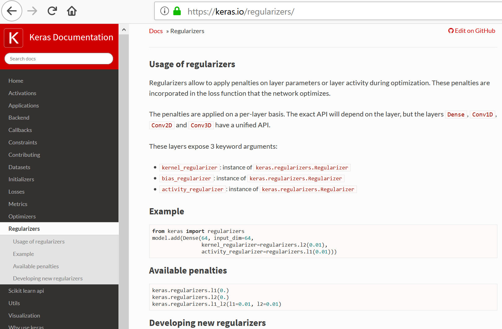
Emirical Risk minimization: $$ f^* = \arg \min\limits_f L_{emp}(f) = \arg \min\limits_f\frac{1}{m}\sum_{i=1}^m L\big(f(\mathbf x_{(i)}), y_i\big) $$ To trade-off model risk and simplicity, we include regularizer: $$ f^* = \arg \min\limits_f \big( L_{emp}(f) + \lambda R(f) \big) = \arg \min\limits_f L_{reg}(f) $$
Just cryptic talk for the same optimization problem we've been doing. But can be extended to cover many different techniques.
Tensor Perspective
Input data $\mathbf x$ can be viewed as vectors, matrices, or beyond... generally called "tensors"
Consider a layer with multiple outputs (e.g. multi-class classifier) $$ f_1(\mathbf x) = \hat{y}_1 \\ f_2(\mathbf x) = \hat{y}_2 \\ ... $$ Layers themselves viewed as functions on tensors.
$$ "\mathbf f(\mathbf x)" = \hat{\mathbf y} $$
Multiple Layers in Tensor perspective
Two-layer network as concatenated single-layer networks: $$ \mathbf f^{(1)}(\mathbf x) = \hat{\mathbf y}^{(1)} \\ \mathbf f^{(2)}(\mathbf x) = \hat{\mathbf y}^{(2)} \\ ... $$ Multilayer network as composition of tensor functions $$ \mathbf f^{(2)}\big(\mathbf f^{(1)}(\mathbf x) \big) = \hat{\mathbf y}^{(2)} \\ $$
Just another model to fit: $$ f_{(entire\_network)}(\mathbf x) = \hat{y} $$
Need to take care that input and output sizes match
Optimize a big Loss function of everything
Loss metrics in Keras
Regularization methods in Keras
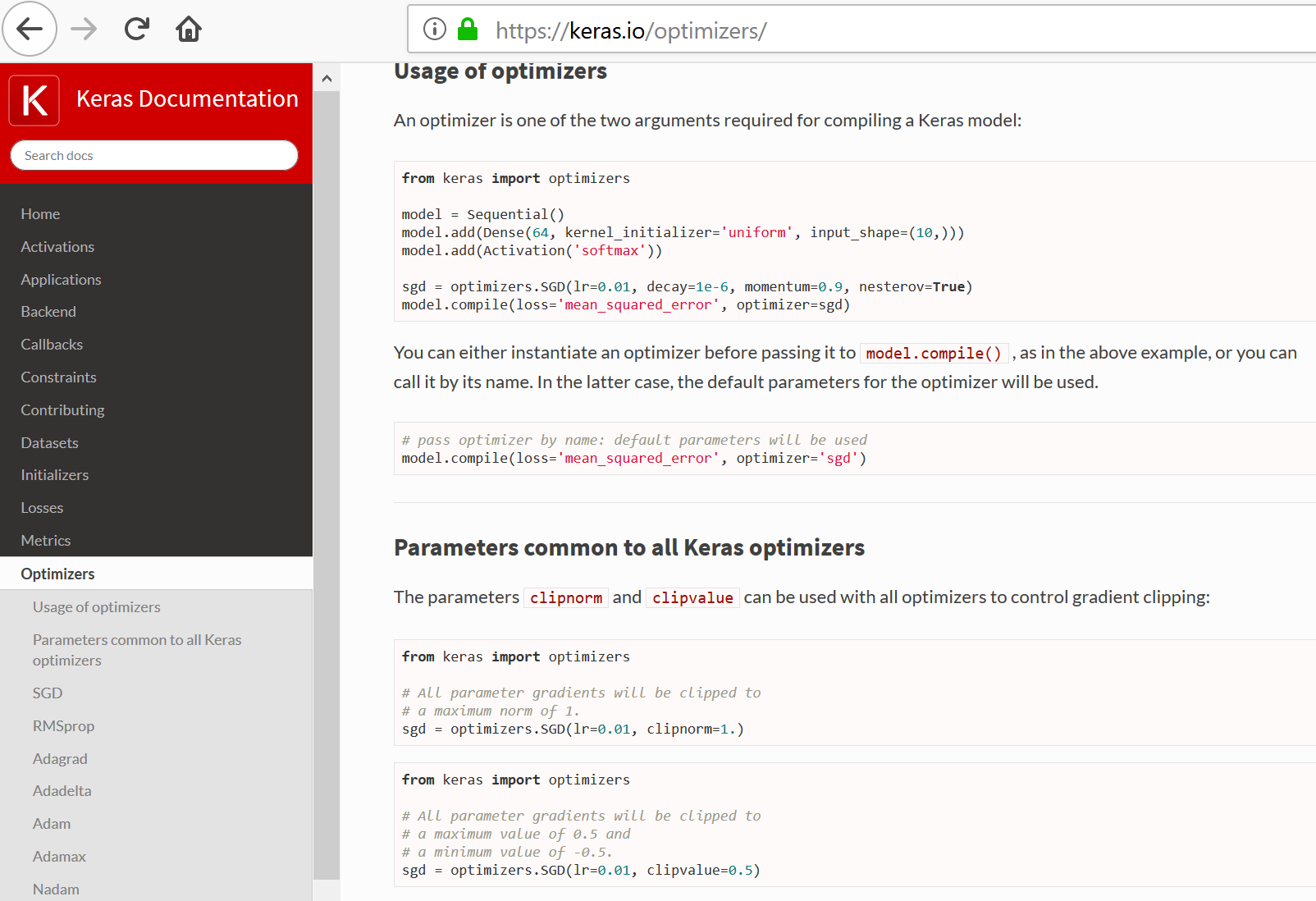
Optimization methods in Keras
Gradient Descent
Went from too-trivial-to-cover in optimization classes, to the current state-of-the-art due to massive data sizes and parallel computing
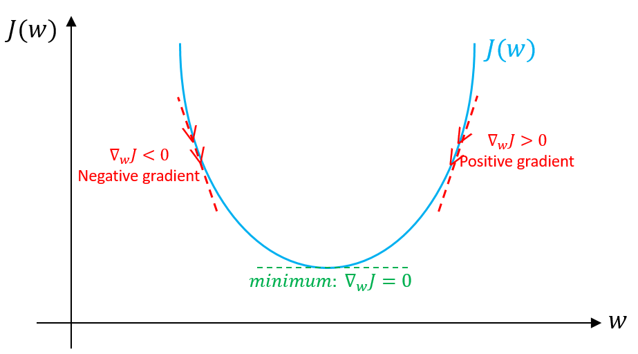
Step size a.k.a. Learning rate.
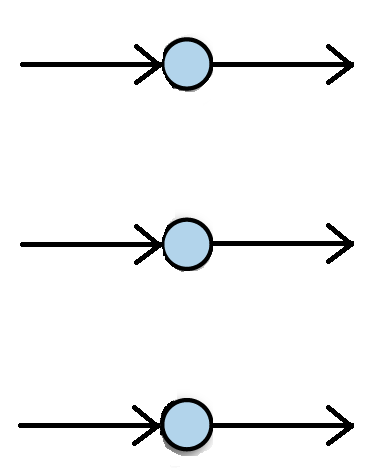
Activation Functions
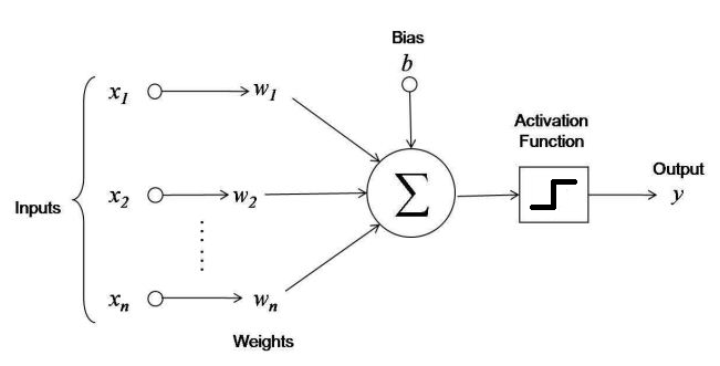
Key nonlinearity needed for Artificial Neural Networks to do anything interesting.
Consider what happens with networks of ANN's with no activation function.
Note these are scalar functions with scalar inputs. First compute the inner product then apply function.
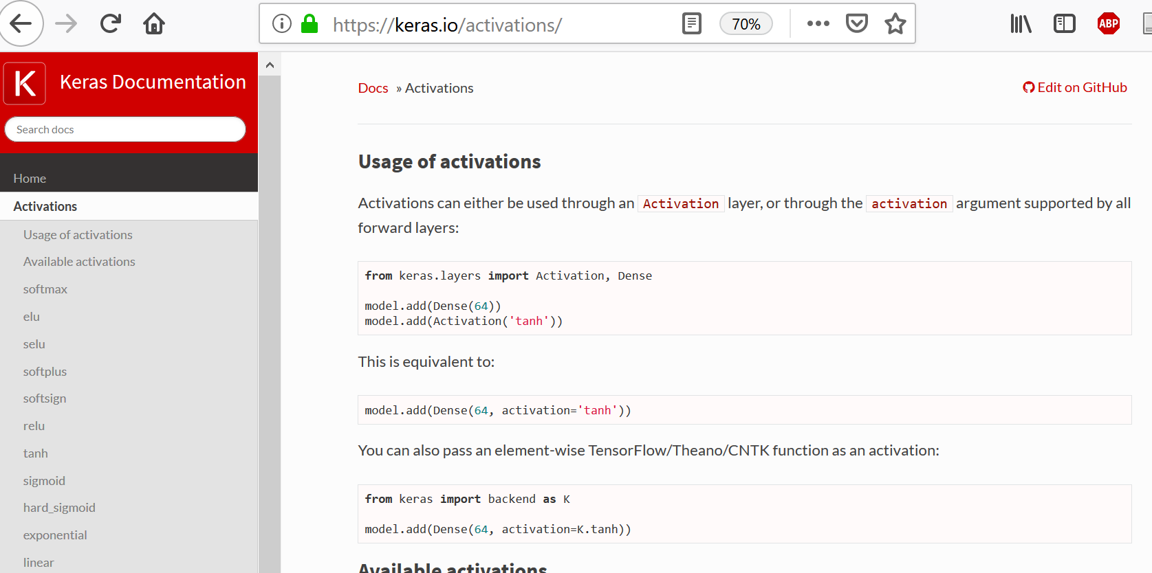
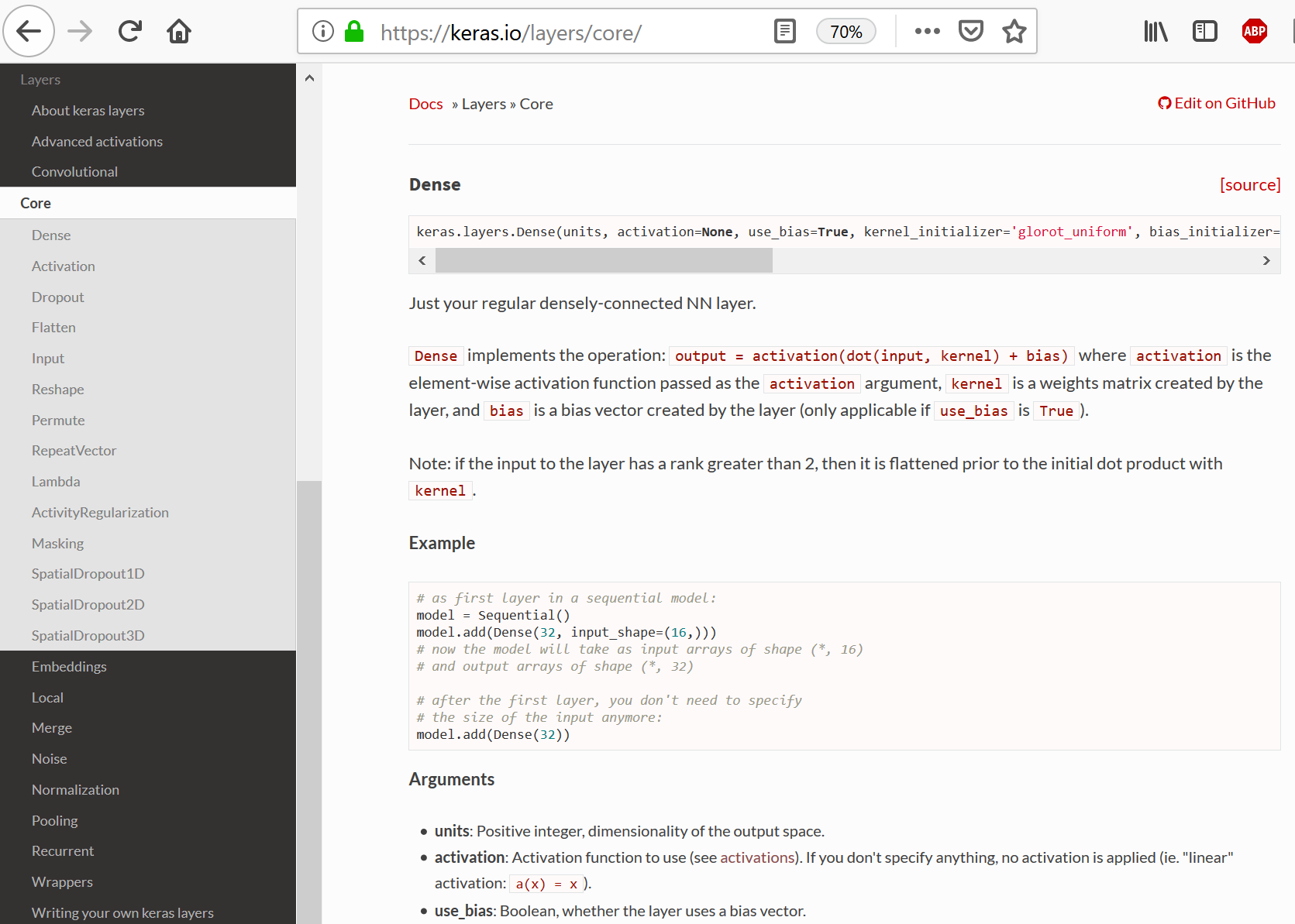
Layers in Keras
Connection decisions: Fully-connected Layers, Convolutional Layers
Unified way to define other aspects of network: activation function, dropout, even pre-processing steps
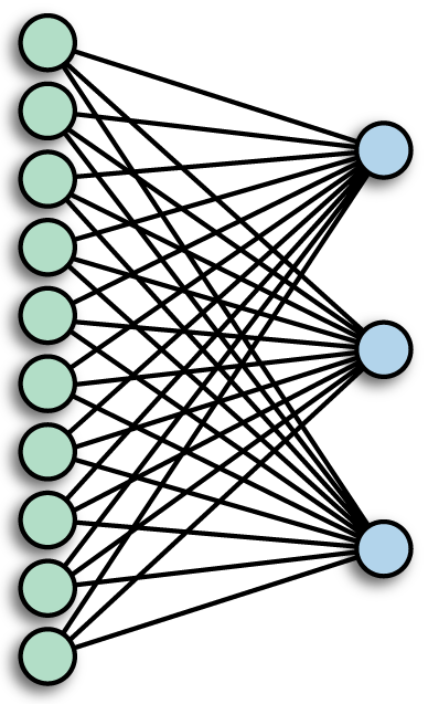
Multilayer (Artificial) Neural Networks - "Feed forward"
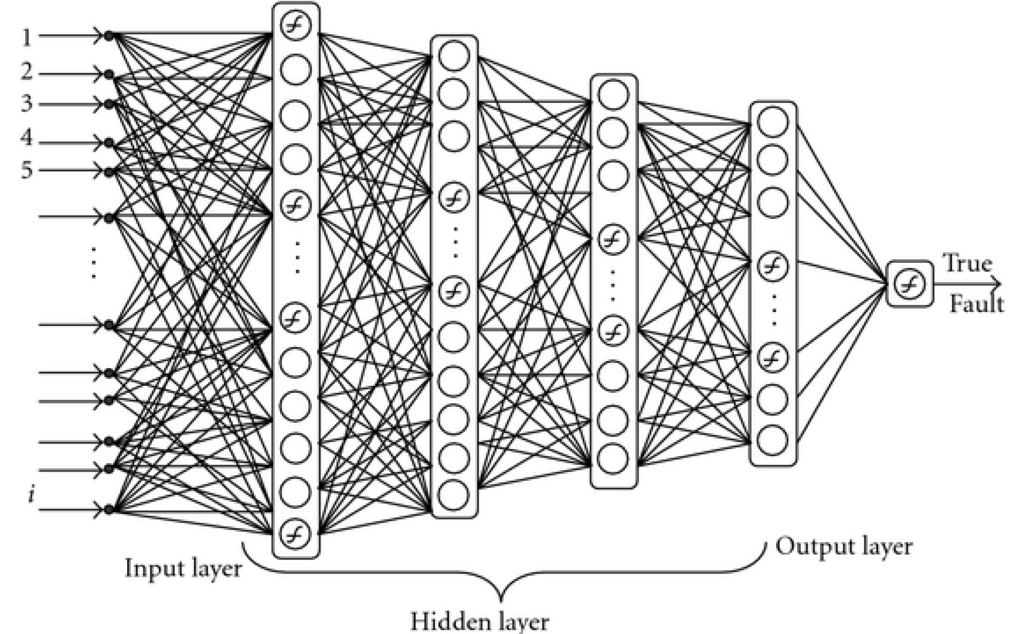
Note each of these is actually two layers in Keras. What kinds are they?
Activation Layer
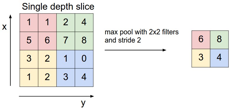
Pooling Layer
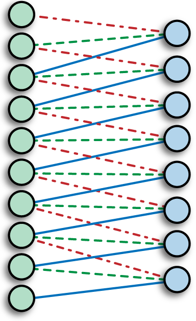
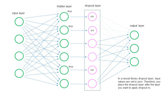
Dropout Layer
Deep Network Design
Make up an architcture - choose layers and their parameters, activation functions, regularization
Choose a Loss function
Choose a optimization method
Choose regularization as optimization options also
Other familiar details like initializing and normalizing data
Keras example
"Deep Learning with Python", Francois Chollet, Ch. 2, https://github.com/fchollet/deep-learning-with-python-notebooks
"Getting Started with TensorFlow and Deep Learning: SciPy 2018 Tutorial", Josh Gordon, https://www.youtube.com/watch?v=tYYVSEHq-io, https://www.tensorflow.org/tutorials/keras/
Train your first neural network: basic classification
https://www.tensorflow.org/tutorials/keras/basic_classification
https://github.com/tensorflow/docs/blob/master/site/en/tutorials/keras/basic_classification.ipynb
# TensorFlow
import tensorflow as tf

print(tf.__version__)
import keras
keras.__version__
fashion_mnist = keras.datasets.fashion_mnist

(train_images, train_labels), (test_images, test_labels) = fashion_mnist.load_data()
class_names = ['T-shirt/top', 'Trouser', 'Pullover', 'Dress', 'Coat',
               'Sandal', 'Shirt', 'Sneaker', 'Bag', 'Ankle boot']

print(train_images.shape)
print(test_images.shape)
print(train_labels)
"Preprocessing"
Note values range from 0 to 255 (8 bit integers)
We want to normalize to between 0 and 1
plt.imshow(train_images[0])
plt.colorbar();

train_images = train_images / 255.0
test_images = test_images / 255.0
plt.figure(figsize=(10,10))
for i in range(25):
    plt.subplot(5,5,i+1)
    plt.xticks([])
    plt.yticks([])
    plt.grid(False)
    plt.imshow(train_images[i], cmap=plt.cm.binary)
    plt.xlabel(class_names[train_labels[i]])

Define the network model
from keras import models
from keras import layers

model = models.Sequential()
model.add(layers.Flatten(input_shape=(28, 28)))
model.add(layers.Dense(128, activation=tf.nn.relu))
model.add(layers.Dense(10, activation=tf.nn.softmax))
model.summary()
"Compile" the network
model.compile(optimizer=tf.train.AdamOptimizer(),
              loss='sparse_categorical_crossentropy',
              metrics=['accuracy'])
- Sparse - recall what this means?
- Cross-entropy
- Categorical Cross-entropy
Optimize the network
model.fit(train_images, train_labels, epochs=5)
Compute accuracy on test set
test_loss, test_acc = model.evaluate(test_images, test_labels)

print('Test accuracy:', test_acc)
Use network to classify samples
predictions = model.predict(test_images)
plt.plot(predictions[1]);

print(np.argmax(predictions[0]), test_labels[0])
print(class_names[np.argmax(predictions[0])], class_names[test_labels[0]])
.predict() expects an array of samples (as a tensor)
img = test_images[0]

print(img.shape)
img_tensor = (np.expand_dims(img,0))

print(img_tensor.shape)
predictions_single = model.predict(img_tensor)

print(predictions_single)
predictions_single = model.predict(np.array([img]))

print(predictions_single)
Adding Validation data
from sklearn.model_selection import train_test_split


X_train, X_valid, y_train, y_valid = train_test_split(test_images, test_labels, test_size=0.33)
model = models.Sequential()
model.add(layers.Flatten(input_shape=(28, 28)))
model.add(layers.Dense(128, activation=tf.nn.relu))
model.add(layers.Dense(10, activation=tf.nn.softmax))

model.compile(optimizer=tf.train.AdamOptimizer(),
              loss='sparse_categorical_crossentropy',
              metrics=['accuracy'])

history =  model.fit(X_train, y_train, validation_data=(X_valid,y_valid), epochs=20)
acc = history.history['acc']
val_acc = history.history['val_acc']
loss = history.history['loss']
val_loss = history.history['val_loss']

epochs = range(len(acc))

plt.plot(epochs, acc, 'bo', label='Training acc')
plt.plot(epochs, val_acc, 'b', label='Validation acc')
plt.title('Training and validation accuracy')
plt.legend()

plt.figure()

plt.plot(epochs, loss, 'bo', label='Training loss')
plt.plot(epochs, val_loss, 'b', label='Validation loss')
plt.title('Training and validation loss')
plt.legend();


Convolutional Network
from keras import layers
from keras import models

model = models.Sequential()
model.add(layers.Conv2D(32, (3, 3), activation='relu', input_shape=(28, 28, 1)))
#model.add(layers.MaxPooling2D((2, 2)))
model.add(layers.Conv2D(64, (3, 3), activation='relu'))
model.add(layers.MaxPooling2D((4, 4)))
model.add(layers.Conv2D(64, (3, 3), activation='relu'))
model.summary()
model.add(layers.Flatten())
#model.add(layers.Dense(64, activation='relu'))
model.add(layers.Dense(10, activation='softmax'))

model.summary()
from keras.datasets import mnist
from keras.utils import to_categorical

(train_images, train_labels), (test_images, test_labels) = mnist.load_data()

train_images = train_images.reshape((60000, 28, 28, 1))
train_images = train_images.astype('float32') / 255

test_images = test_images.reshape((10000, 28, 28, 1))
test_images = test_images.astype('float32') / 255

train_labels = to_categorical(train_labels)
test_labels = to_categorical(test_labels)
model.compile(optimizer='rmsprop',
              loss='categorical_crossentropy',
              metrics=['accuracy'])
model.fit(train_images, train_labels, epochs=5, batch_size=64)
test_loss, test_acc = model.evaluate(test_images, test_labels)
test_acc