Unstructured Data & Natural Language Processing

Keith Dillon
Spring 2020

Topic 4: Probabilistic Modeling

This topic:

1. Probability Review
2. $N$-gram Language modeling
3. Naive Bayes
4. Logistic Regression

Reading:

• J&M Chapter 3 (Language Modeling with N-Grams)
• J&M Chapter 4 (Naive Bayes Classification and Sentiment)
• J&M Chapter 5 (Logistic Regression)

I. Probability Review

http://j.mp/CG_prob_cheatsheet

Sample space

$\Omega$ = set of all possible outcomes of an experiment

Examples:

• $\Omega = \{HH, \ HT, \ TH, \ TT\}$ (discrete, finite)
• $\Omega = \{0, \ 1, \ 2, \ \dots\}$ (discrete, infinite)
• $\Omega = [0, \ 1]$ (continuous, infinite)
• $\Omega = \{ [0, 90), [90, 360) \}$ (discrete, finite)

Events

subset of the sample space. That is, any collection of outcomes forms an event.

Example:

Toss a coin twice. Sample space: $\Omega = \{HH, \ HT, \ TH, \ TT\}$

Let event $A$ be the event that there is exactly one head

We write: $A =“exactly \ one \ head”$

Then $A = \{HT, \ TH \}$

$A$ is a subset of $\Omega$, and we write $A \subset \Omega$

Combining Events: Union, Intersection and Complement

• Union of two events $A$ and $B$, called $A \cup B$ = the set of outcomes that belong either to $A$, to $B$, or to both. In words, $A \cup B$ means "A or B."
• Intersection of two events $A$ and $B$, called $A \cap B$ = the set of outcomes that belong both to $A$ and to $B$. In words, $A \cap B$ means “A and B.”
• Complement of an event $A$, called $A^c$ = the set of outcomes that do not belong to $A$. In words, $A^c$ means "not A."

Theorems:

• The probability of event "not A": $P(A^c) = 1 - P(A)$
• For any A and B (not necessarily disjoint): $P(A \cup B) = P(A) + P(B) - P(A \cap B)$

Notation note: $P(A,B) = P(A \text{ AND } B) = P(A \cap B)$

Venn Diagram

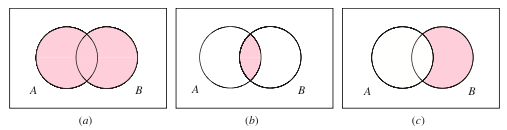
This sort of diagram representing events in a sample space is called a Venn diagram.

a) $A \cup B\quad(e.g. 6$ on either $die_1$ or $die_2$ (or both)$)$
b) $A \cap B\quad(e.g. 6$ on both $die_1$ and $die_2)$
c) $B \cap A^c\quad(e.g. 6$ on $die_2$ but not on $die_1)$

Axioms of Probability

• For any event $A$: $P(A) \geq 0$
• The probability of the entire sample space: $P(\Omega) = 1$
• For any countable collection $A_1, A_2,...$ of mutually exclusive events:
  $$P(A_1\cup A_2 \cup \dots) = P(A_1) + P(A_2) + \dots$$

Independent Events

Events A and B are independent if and only if: $P(A \cap B) = P(A)P(B)$

Question:

What are the probablities of the two events?

• rolling at least one six in 4 throws of a single die
• rolling at least one double six in 24 throws of a pair of dice

Law of Total Probability

If $B_1, B_2, \dots, B_k$ form a partition of $\Omega$, then $(A \cap B_1), (A \cap B_2), \dots, (A \cap B_k)$ form a partition of the set or event A.

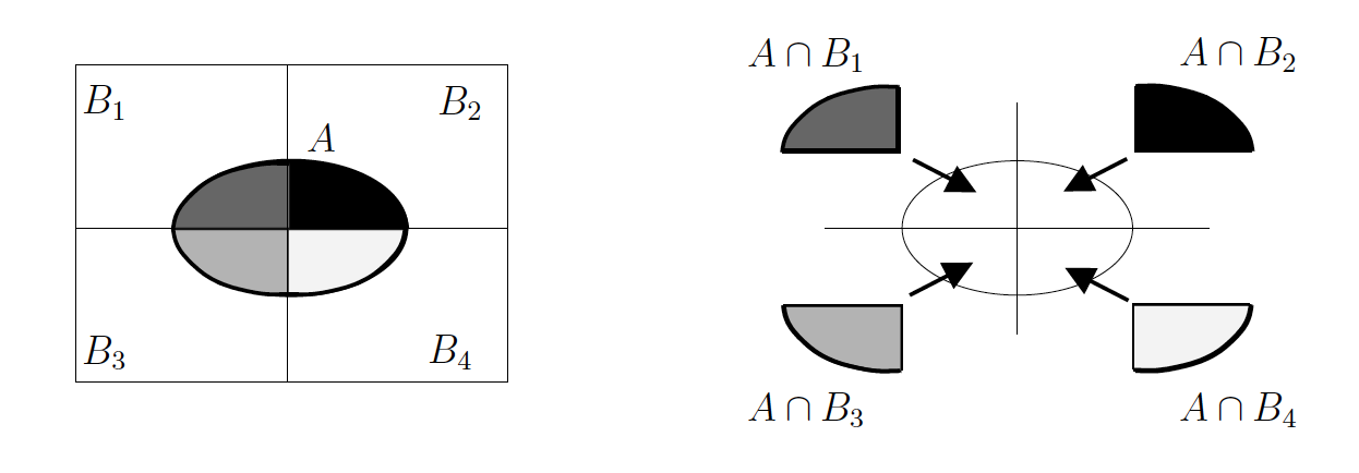
The probability of event A is therefore the sum of its parts:

$$P(A) = P(A \cap B_1) + P(A \cap B_2) + P(A \cap B_3) + P(A \cap B_4)$$

Counting

If experiment $A$ has $n$ possible outcomes, and experiment $B$ has $k$ possible outcomes, then there are $nk$ possible outcomes when you perform both experiments.

Example:

Let $A$ be the experiment "Flip a coin." Let $B$ be "Roll a die." Then $A$ has two outcomes, $H$ and $T$, and $B$ has six outcomes, $1,...,6$. The joint experiment, called "Flip a coin and roll a die" has how many outcomes?

Theorem

Given $n$ distinguishable objects, there are $n^k$ ways to choose a sample of $k$ objects with replacement.

Example:

How many ways are there to sample 5 students out of 20 with replacement?

Explain what this computation means in this case

Permutation

• The number of $k$-permutations of $n$ distinguishable objects is $$^nP_k=n(n-1)(n-2)\dots(n-k+1) = \frac{n!}{(n-k)!}$$

• The number of ways to select $k$ objects from $n$ distinct objects when different orderings constitute different choices

Example

I have five vases, and I want to put two of them on the table, how many different ways are there to arrange the vases?

Combination

If order doesn't matter...

• The number of ways to choose $k$ objects out of $n$ distinguishable objects is $$ ^nC_k = \binom{n}{k} = \frac{^nP_k}{k!}=\frac{n!}{k!(n-k)!}$$

Example

Q. How many ways are there to get 4 of a kind in a 5 card draw?

A. Break it down:

1. Q. How many ways are there to get 4 of a kind?
   A. $\binom{13}{1}$
2. Q. How many ways can you fill the last card?
   A. $\binom{52-4}{1}$
3. Total: $$\binom{13}{1} \binom{48}{1} = 13 \times 48 = 624$$

Example

Q. How many ways are there to get a full house in a 5 card draw?

A. The matching triple can be any of 13 the denominations and the pair can be any of the remaining 12 denominations.

1. Q. How many ways are there to select the suits of the matching triple?
   A. $13\binom{4}{3}$
2. Q. How many ways are there to select the suits of the matching pair?
   A. $12\binom{4}{2}$
3. Total: $$13\binom{4}{3} \times 12\binom{4}{2} = 13 \times 4 \times 12 \times 6 = 3,744$$

Conditional Probability: The probability that A occurs, given B has occurred

$$ P(A|B) = \frac{P(A\cap B)}{P(B)} $$

Joint probability: $P(A \cap B) = P(A|B) \times P(B)$

Law of Total Probability: If $B_1, \dots, B_k$ partition $S$, then for any event A,

$$ P(A) = \sum_{i = 1}^k P(A \cap B_i) = \sum_{i = 1}^k P(A | B_i) P(B_i) $$

Bayes' Theorem :

$$ P(A|B) = \frac{P(B|A) \times P(A)}{P(B)} = \frac{P(B|A) \times P(A)}{P(B|A) \times P(A) + P(B|A^c) \times P(A^c)} $$

Chain Rule for Probability

We can write any joint probability as incremental product of conditional probabilities,

$ P(A_1 \cap A_2) = P(A_1)P(A_2 | A_1) $

$ P(A_1 \cap A_2 \cap A_3) = P(A_1)P(A_2 | A_1)P(A_3 | A_2 \cap A_1) $

In general, for $n$ events $A_1, A_2, \dots, A_n$, we have

$ P (A_1 \cap A_2 \cap \dots \cap A_n) = P(A_1)P(A_2 | A_1) \dots P(A_n | A_{n-1} \cap \dots \cap A_1) $

Estimating probabilities

Frequentist perspective: probability of event is relative frequency

$$P(A) = \frac{\text{# times $A$ occurs}}{\text{total # experiments}}$$

$$P(A,B) = \frac{\text{# times $A$ and $B$ occur together}}{\text{total # experiments}}$$

$$P(A|B) = \text{?}$$

Problems with relative frequency

1. Sampling may not be sufficently random (or large number).

$$P(\text{candidate will win}) = \frac{\text{# facebook users who support candidate}}{\text{total # of facebook users}}?$$

1. Very rare events.

$$P(\text{winning lottery}) = \frac{\text{# times won lottery}}{\text{total # times bought ticket}} = 0?$$

II. Language Modeling

(Probabilistic) Language Modeling (LM)

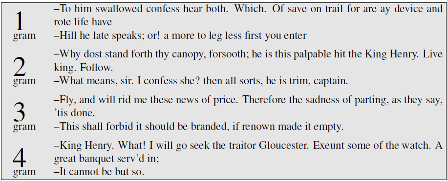
Assign probabilities to sequences of "words". This is a model of language structure.

Most common word is "the"

Is the most common two-word sentence therefore: "the the."?

Spelling & grammar correction: "Their are problems wit this sentence"

"Their are..." vs. "There are..." vs. "They're are..."

Predict next word in this sequence: "5, 4, 3, 2, _"

Speech recognition: “I ate a cherry” or “Eye eight uh Jerry”

Automatic translation (that makes sense)

他向记者介绍了发言的主要内容

1. He briefed to reporters on the chief contents of the statement
2. He briefed reporters on the chief contents of the statement
3. He briefed to reporters on the main contents of the statement
4. He briefed reporters on the main contents of the statement

"Sequence" model

$$P(\text{first word}=\text{"once"},\text{second word}=\text{"upon"},\text{third word}=\text{"a"},\text{fourth word}=\text{"time"})$$

Or with vector notation $P(\mathbf w)$, where $w_1$="once", $w_2$="upon", $w_3$="a", $w_4$="time".

Note these are not quite the same as the simple joint probability of the words, i.e.,

$$P(\text{"once"},\text{"upon"},\text{"a"},\text{"time"}) = P(\text{"upon"},\text{"a"},\text{"time"},\text{"once"}) = ...$$

Unless we choose to ignore relative location of words (will get to that soon).

"Predictive" model

$$P(\text{fourth word}=\text{"time"}\,|\,\text{first word}=\text{"once"},\text{second word}=\text{"upon"},\text{third word}=\text{"a"})$$

Different versions of same information. Both are referred to as "language models".

Estimating sentence probabilities

$$P(\text{"The cat sat on the hat."}) = \frac{\text{# times corpus contains sentence: "The cat sat on the hat."}}{\text{total # of sentences in corpus}}?$$$$P(\text{"...hat"} \,|\, \text{"The cat sat on the..."}) = ?$$

$$ P(A|B) = \frac{P(A\cap B)}{P(B)} $$

$$P(\text{"...hat"} \,|\, \text{"The cat sat on the..."}) = \frac{\text{# times corpus contains sentence: "The cat sat on the hat."}}{\text{# of sentences starting with "The cat sat on the..."}}?$$

Problem: most sentences will never appear in our corpus.

Exercise: Rare sentences

We need to assign a probability to every possible sentence

Suppose our vocubulary is (limited to) 10,000 words

How many possible 5-word sentences are there?

$(10,000)^5 = 10^{20}$ -- sampling with replacement

Multivariate vs Joint Probability

We consider a sequence of words as a vector (really a list of strings here)

$$ \mathbf w = (w_1, w_2, ..., w_n)$$$$ w_1 = "the", \, w_2 = "cat",\, w_3 = "sat", \, ... $$

Position is important. What are the events?

$P(W = \mathbf w)$ is the probability that the random variable $W$ takes the value $\mathbf w$ (our vector)

J&M also writes this as

$$P(w_1 w_2 ... w_n)$$

Note this is not a product.

Think of $P(w_1 w_2 ... w_n)$ as $P(W_1 = w_1, W_2=w_2, ..., W_n = w_n)$, a multivariate distribution.

Sometimes we may get sloppy with the notation. Generally expect order to matter unless we are doing a method where we discard info about order.

Relating joint probability $P(w_1w_2w_3)$ to conditional $P(w_3|w_1w_2)$

How do we do this?

Answer: use the Chain Rule of Probability

The chain rule of probability

$$P(w_1w_2) = P(w_2|w_1)P(w_1)$$$$P(\text{"the cat"}) = P(\text{"...cat"}|\text{"the..."})P(\text{"the..."})$$

$$P(w_1w_2w_3) = P(w_3|w_1w_2)P(w_1w_2)$$\begin{align} P(\text{"the cat sat"}) &= P(\text{"...sat"}|\text{"the cat..."})P(\text{"the cat..."}) \\ &=P(\text{"...sat"}|\text{"the cat..."})P(\text{"...cat..."}|\text{"the..."})P(\text{"the..."}) \end{align}

The chain rule of probability

\begin{align} P(w_1w_2...w_n) &= P(w_n|w_{n-1}...w_1)P(w_{n-1}|w_{n-2}...w_1)...P(w_1) \\ &= \prod_{k=1}^n P(w_k|w^{k-1}_1) \end{align}

where $w^{b}_a \equiv w_aw_{a+1}...w_b$.

$N$-grams

Model order limited to length $N$ sequences:

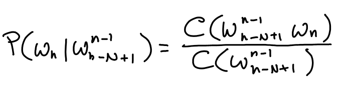
\begin{align} P(w_n|w_{n-1}...w_1) &\approx P(w_n|w_{n-1}...w_{n-(N-1)}) \\ P(w_n|w^{n-1}_1) &\approx P(w_n|w^{n-1}_{n-N+1}) \end{align}

So use previous $N-1$ words.

1. Unigram
2. Bigram
3. Trigram

Exercise: list all possible bigrams from sentence "The cat sat on the hat."

Exercise: list all possible unigrams.

https://ai.googleblog.com/2010/12/find-out-whats-in-word-or-five-with.html

Bag-of-Words (BOW)

Convert a text string (like a document) into a vector of word frequencies by essentially summing up the one-hot encoded vectors for the words. Perhaps divide by total number of words.

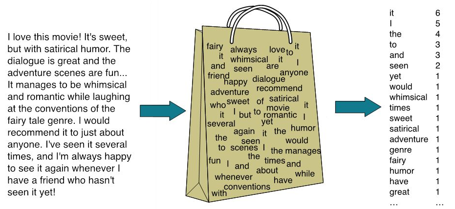
Basically get histogram for each documents to use as feature vectors. Becomes structured data.

What kind of $N$-gram does this use?

Markov assumption

Future state only depends on present state (not past states)

How might this apply to word prediction?

$$P(\text{word}\,|\,\text{all previous words}) = P(\text{word}\,|\,\text{immediately preceding word only})$$

What kind of $N$-gram does this use?

First-order Markov process

An initial distribution over states and a state transition matrix

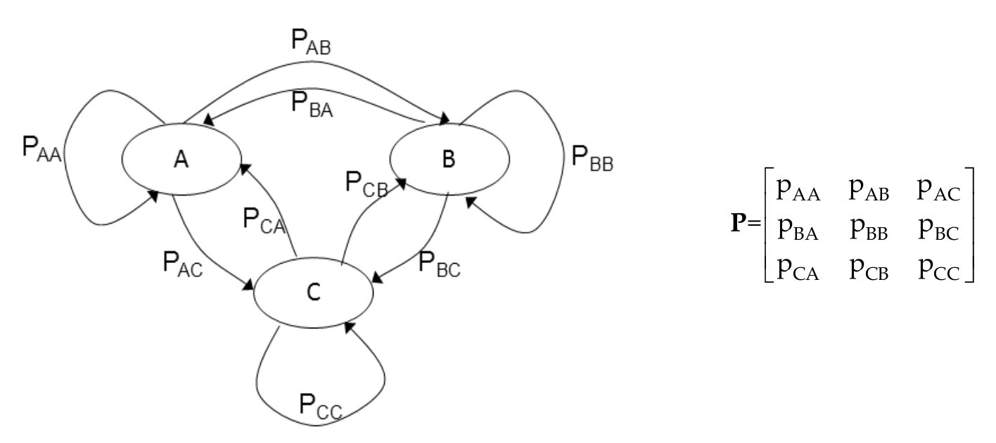
Higher-order Markov processes. Probability of next step depends on current node and previous node.

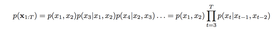
$N$-grams for $N>2$

Bigram Probability Estimation

Using the Law of Total Probability

What is P(<s>|</s>)?

What is the P(eggs|green)?

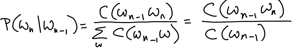
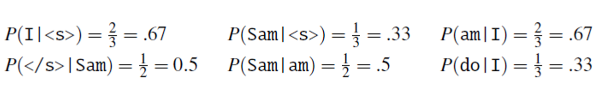
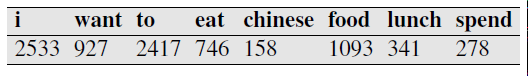
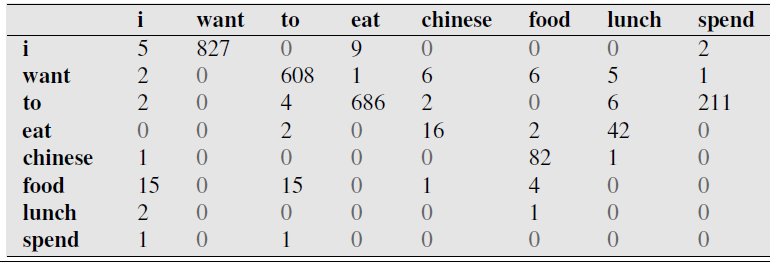
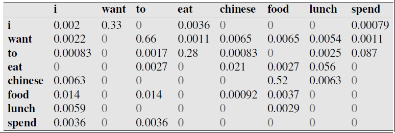
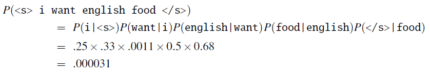
$N$-gram Probability Estimation

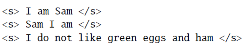
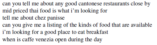
Bigram Example - Berkeley Restaurant database

Notes

• Trigrams are actually much more commonly used in practice, but bigrams easier for examples

• In practice, we work with log-probabilities instead to avoid underflow

Exercise: demonstrate how this calculation would be done with log-probabilities

Model Evaluation

• Extrinsic versus Intrinsic

• Training set, Test set, and "Dev Set"

Use Training Set for computing counts of sequences, then compare to Test set.

Perplexity of a Language Model (PP)

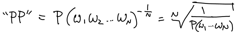
Bigram version:

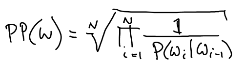
Weighted average branching factor - number of words that can follow any given word, weighted by probability.

Note similarity to concept of information entropy.

Exercise: perplexity of digits

1. Assume each digit has probability of $\frac{1}{10}$, independent of prior digit. Compute PP.

2. What happens if probabilities vary from this uniform case?

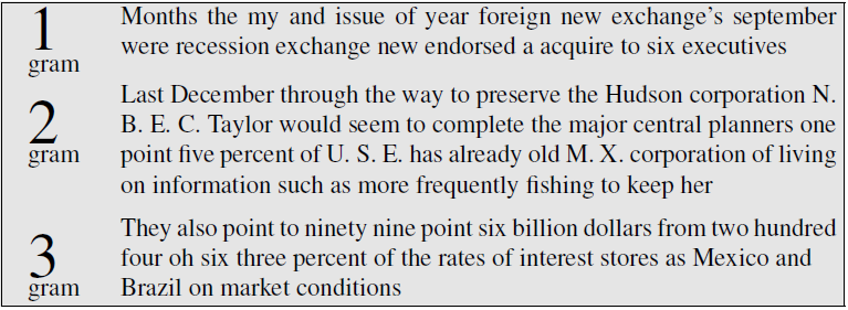
Perplexity for comparing $N$-gram models

WSJ dataset: 20k word vocabulary, 1.5M word corpus.

• Unigram Perplexity: 962
• Bigram Perplexity: 170
• Trigram Perplexity: 109

Perplexity Notes

• Overfitting and Bias cause misleadingly low PP

• Shorter vocabulary causes higher PP, must compare using same size.

Evaluating $N$-grams with randomly-generated sentences

Using Shakespeare corpus:

Using WSJ treebank corpus:

Note bias caused by corpus, inportance of genre & dialect.

Sparse $N$-gram problem

Consider what happens to this calculation if any of our $N$-gram count are zero in the corpus.

Closed Vocabulary System - Vocabulary is limited to certain words. Ex: phone system with limited options.

Open Vocabulary System - Possible unknown words - set to . Typically treat as any other word.

Out-of-Vocabulary (OOV) - words encoutered in test set (or real application) which aren't in training set.

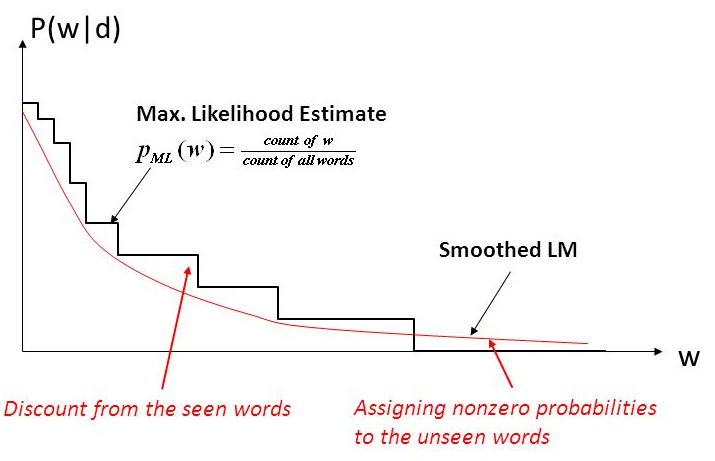
Smoothing a.k.a. Discounting

Adjust $N$-gram counts to give positive numbers in place of zeros, reduces counts of others.

Laplace a.k.a. Additive smoothing

https://en.wikipedia.org/wiki/Additive_smoothing

$$P(w_i) = \dfrac{C(w_i)}{N} \approx \dfrac{C(w_i)+1}{N+V}$$

$N$ = total number of words.

$V$ = size of vocabulary.

Adjusted count: $C^*(w_i) = \left(C(w_i)+1\right)\dfrac{N}{N+V}$

Exercise: compute $P(w_i)$ using the adjusted count.

Discount = reduction for words with nonzero counts = $d_c=\dfrac{C^*(w_i)}{C(w_i)}$

Before Laplace smoothing:

After Laplace smoothing:

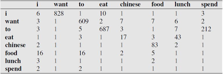
Before Laplace smoothing:

After Laplace smoothing:

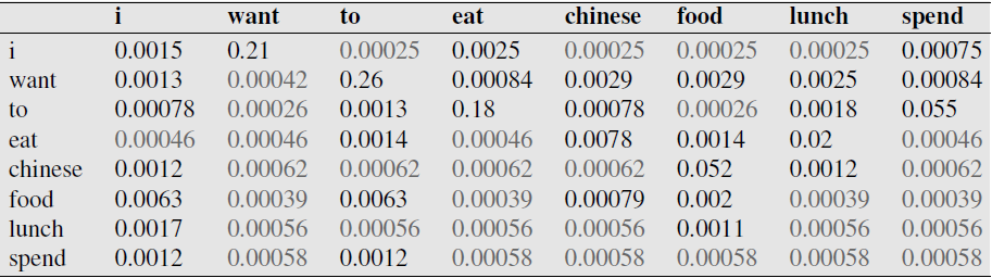
Note large reductions.

Backoff: If desired $N$-gram not available, use $(N-1)$-gram.

Stupid Backoff: perform backoff but don't bother adjusting normalization properly.

Interpolation: combine $N$-grams for different $N$.

Simple linear interpolation: linear combination of $N$-gram with $(N-1)$-gram and $(N-2)$-gram ... and unigram.

Weights are hyperparameters, sum to one.

Note need to adjust normalization (denominator in probability estimate) depending on total number $N$-grams used

Absolute Discounting

Church & Gale noticed in 1991 using AP Newswire dataset with 22M word training set and 22M word test set:

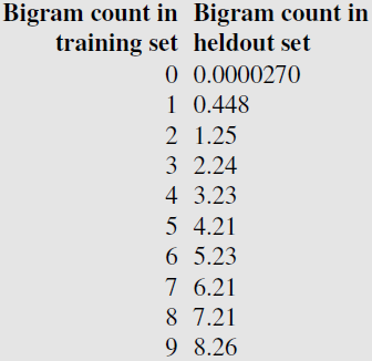
Bigram Absolute discounting with interpolated Backoff

$$ P_{Abs}(w_i|w_{i-1})= \dfrac{C(w_{i-1}w_i)-d}{\sum_vC(w_{1-1}v)}+\lambda(w_{i-1})P(w_i) $$

context-dependent weights: $\lambda$ higher when count higher.

Continuation Probability

Consider $P(\text{kong})>P(\text{glasses})$, but $P(\text{reading glasses})>P(\text{reading kong})$

Bigrams should capture this, but when we don't have any in training set and need to do backoff, want to still maintain the effect.

Replace unigram probability with continuation probability.

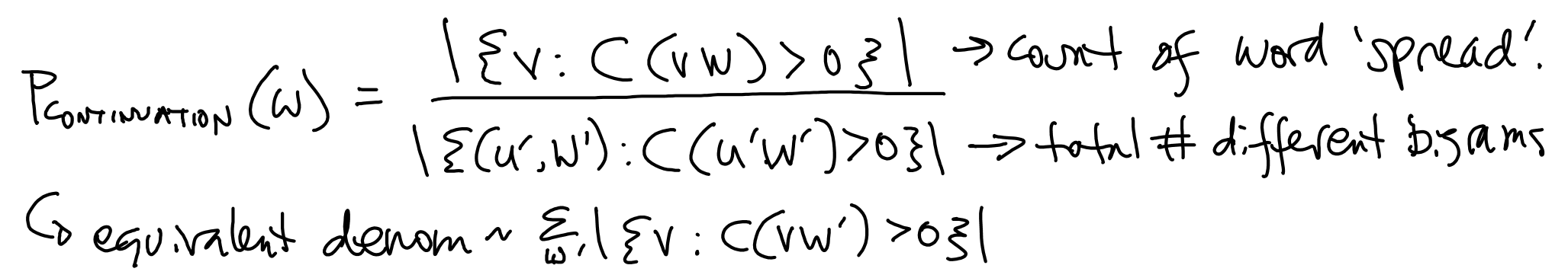
Word appears in many different bigrams --> higher $P_{CONTINUATION}$

Kneser-Ney Smoothing

Use absolute smoothing

Uses continuation probability for low counts

Bigram version:

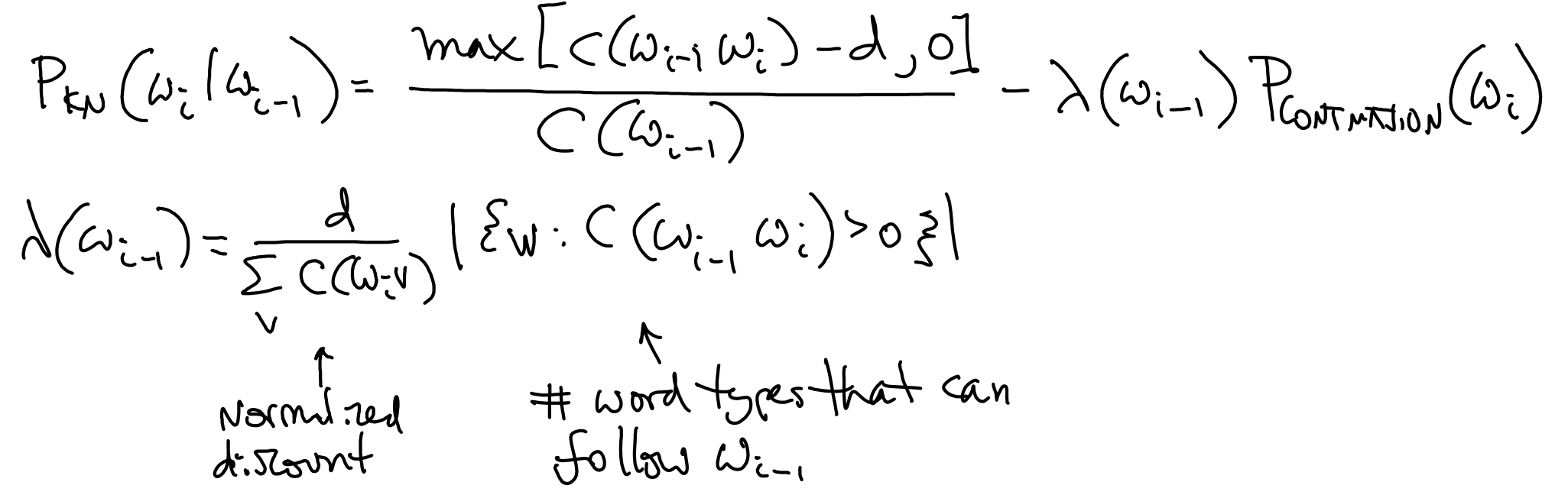
Recursive implementation for $N$-grams.

III. Naive Bayes Classification

Text Categorization

the task of assigning a label or categorization category to an entire text or document

• sentiment analysis - positive or negative orientation that a writer expresses toward some object. A review of a movie, book, or product on the web expresses the author’s sentiment toward the product, while an editorial or political text expresses sentiment toward a candidate or political action.
• spam detection
• language identification
• authorship attribution
• topic classification

Example: sentiment analysis

Words like great, richly, awesome, and pathetic, and awful and ridiculously are very informative cues:

• • ...zany characters and richly applied satire, and some great plot twists
• • It was pathetic. The worst part about it was the boxing scenes...
• • ...awesome caramel sauce and sweet toasty almonds. I love this place!
• • ...awful pizza and ridiculously overpriced...

(so a unigram model might work reasonably well)

Supervised machine learning

• have a data set of input observations, each associated with some correct output (a ‘supervision signal’).
• The goal of the algorithm is to learn how to map from a new observation to a correct output.
• Input: $x$, a.k.a. $d$ (document)
• Output: $y$, a.k.a. $c$ (class)

• Probabilistic classifier: output class probabilities, e.g. 99% chance of belonging to class 0, 1% to class 1.
• Generative classifiers: model data generated by class. Then use it to return class most likely to have generated data. Ex: Naive Bayes.
• Discriminative classifiers: learn model to directly discriminate classes given data, ex. logistic regression.

Naive Bayes = MAP estimate of class

\begin{align} \hat{c} &= \arg \max_c P(c|d) \\ &= \arg\max_c \dfrac{P(d|c)P(c)}{P(d)} \\ &= \arg\max_c P(d|c)P(c) \end{align}

$P(c|d)$ = posterior probability

$P(d|c)$ = likelihood of data

$P(c)$ = prior probability of class $c$

Naive assumption

\begin{align} P(d|c) &= P(w_1w_2...w_L|c) \\ &\approx P(w_1|c)P(w_2|c)...P(w_L|c) \end{align}

\begin{align} \arg\max_c P(d|c)P(c) \rightarrow \arg \max_c P(w_1|c)P(w_2|c)...P(w_L|c)P(c) \end{align}

Inference using model

$$ c_{NB} = \arg\max_c P(c) \prod_i P(w_i|c) $$

Where the product index $i$ runs over every word in document (including repeats).

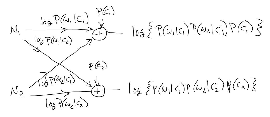
Using log-probabilities

$$ c_{NB} = \arg\max_c \left\{ \log P(c) + \sum_i \log P(w_i|c) \right\} $$

Note this can be viewed as a linear classification technique, take linear combination by applying weight to each feature (word).

Feature vector as list of 1's. Different weight vector for each class, document-specific.

Or with bag-of-words representation, feature vector as histogram. Can apply same weight vectors to different documents.

\begin{align} c_{NB} &= \arg\max_c \left\{ \log P(c) + \sum_i \log P(w_i|c) \right\} \\ &= \arg\max_c \left\{ \log P(c) + \sum_{w \in V} N_w \log P(w|c) \right\} \\ \end{align}

where we sum over all words in vocabulary, and apply weights.

Note that outputs aren't class probabilities. How could we make them into probabilities?

Bag-of-Words (BOW)

Convert a text string (like a document) into a vector of word frequencies $(N_1,N_2, ...)$ by essentially summing up the one-hot encoded vectors for the words. Perhaps divide by total number of words.

Basically get histogram for each documents to use as feature vectors. Becomes structured data.

How does this relate to $N$-grams?

Estimating the probabilities

$$ P(c) = \text{probability of document belonging to class $c$} \approx \dfrac{\text{# documents in corpus belonging to class $c$}}{\text{total # documents in corpus}} $$

$$ P(w|c) = \text{probability of word $w$ appearing in document from class $c$} \approx \dfrac{\text{count of word $w$ in documents of class $c$}}{\text{total # words in documents of class $c$}} $$

What probability rule are we using here?

Application notes

• Need smoothing (Laplace is popular for this Naive Bayes) for dealing with zeros.
• Unknown words typically can be ignored here.
• Stop words and frequent words like 'a' and 'the' also often ignored.
• special handling of negation for sentiment applications - include negated versions of words

Binary Naive Bayes: rather than using counts (and smoothing), just use binary indicator of word presense or absense (1 or 2, rather than 0 or 1, to avoid zeros). Essentially just remove word repeats from document.

Get word classes from online lexicons

Lists of positive vs negative words.

• General Inquirer (Stone et al., 1966),
• LIWC (Pennebaker et al., 2007),
• the opinion lexicon of Hu and Liu (2004a)
• the MPQA Subjectivity Lexicon (Wilson et al., 2005).

Summary: Naive Bayes versus Language Models

A language model models statistical relationsips between words, can be used to predict words of high overall probability for a string of text.

Naive bayes models statistical relationships between words and classes. Used to predict a class given words.

IV. Logistic Regression

Logistic Regression... Classification

• A key baseline approach for ML in NLP
• Scalable - simply a shallow (i.e., no hidden layers) neural network with sigmoid activation