Unstructured Data & Natural Language Processing

Topic 5: "Vector Embeddings"

This topic:

1. Vector Semantics
2. Dimensionality Reduction
3. Word Embeddings

Reading:

• Alpaydin Chapter 6 (Dimensionality Reduction)
• J&M Chapter 6. (Vector Semantics)

I. Vector Semantics

Motivation

The representation of text (words, sentences, documents, etc.) with vectors

This allows geometric analysis of these vectors (e.g. words may be close, far away, etc, as computed via distance metrics on the vectors).

Distributional hypothesis - Words that occur in similar contexts tend to have similar meanings.... so close together in a gometric sense.

Synonyms (like oculist and eye-doctor) tended to occur in the same environment (e.g., near words like eye or examined) with the amount of meaning difference between two words “corresponding roughly to the amount of difference in their environments” (Harris, 1954, 157).

Vector semantics

• a model which instantiates this linguistic hypothesis by learning representations of the meaning of words directly from their distributions in texts.
• example of representation learning

Lexical Semantics - The linguistic study of word meanings

Lemma

word at top of definition, main representative form chosen. "Citation form".

mouse (N)
    1. any of numerous small rodents...
    2. a hand-operated device that controls a cursor...

Wordforms - other forms of lemma, such as "mice".

Word sense - the meaning(s) of the lemma

Synonym - words with same word sense. couch/sofa.

Antonyms - words with an opposite meaning. long/short.

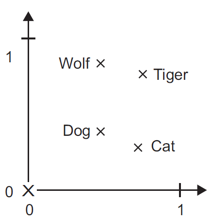
Word Similarity

Some degree of similarity exists for many words with different meanings. Cat vs. Dog. See vs. Hear.

SimLex-999 dataset (Hill et al., 2015) gives values on a scale from 0 to 10, like the examples below, which range from near-synonyms (vanish, disappear) to pairs that scarcely seem to have anything in common (hole, agreement). Judged by humans.

Word relatedness, a.k.a. association

E.g., Coffee vs. cup

Multiple kinds of relatedness.

• Semantic field - topic relatedness. scalpel/surgeon/nurse.
• Semantic frame - different perspectives of same thing. buy/sell/pay/customer
• Taxonomic - subclass. animal/dog.

Connotation

Affective meaning, i.e., emotion/sentiment

Dimensions:

• valence: the pleasantness of the stimulus - happy vs. unhappy
• arousal: the intensity of emotion provoked by the stimulus - excited vs. calm
• dominance: the degree of control exerted by the stimulus

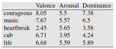
Word as a coordinate in 3D space.

Historical Vector Semantics

1950's: define word as distribution over contexts, the neighboring words or grammatical environments.

Ex: ongchoi (Cantonese). Given contexts:

(6.1) Ongchoi is delicious sauteed with garlic.
(6.2) Ongchoi is superb over rice.
(6.3) ...ongchoi leaves with salty sauces...

And given other contexts of the neighboring words.

(6.4) ...spinach sauteed with garlic over rice...
(6.5) ...chard stems and leaves are delicious...
(6.6) ...collard greens and other salty leafy greens

Conclusion: onchoi is similar to spinach & collard greens.

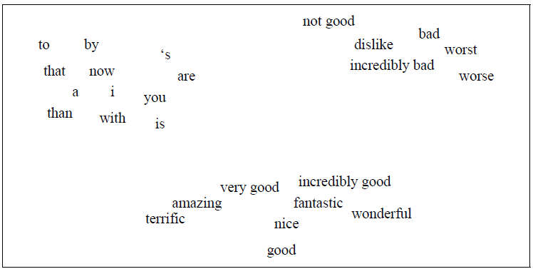
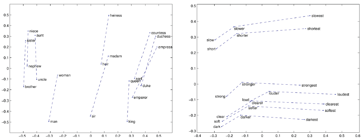
Figure 6.1 A two-dimensional (t-SNE) projection of embeddings for some words and phrases, showing that words with similar meanings are nearby in space. The original 60- dimensional embeddings were trained for a sentiment analysis task. Simplified from Li et al. (2015).

Vector semantic models

• Embeddings of word in a particular vector space
• Better handle OOV words, only need similar words in training set
• Can be learned automatically from text without any complex labeling or supervision.
• Now the standard way to represent the meaning of words in NLP

Will cover two models: tf-idf and word2vec

Term-document matrix

A kind of co-occurence matrix, which counts how ofen words co-occur based on being in the same context or document. BOW representation of documents.

Figure 6.2 The term-document matrix for four words in four Shakespeare plays. Each cell contains the number of times the (row) word occurs in the (column) document.

Dimensionality of vectors is number of words used, here 4. Equal to vocabulary size used.

Gigantic matrix for all words $\times$ all documents. Exploit sparsity.

Document vectors

Used in Information Retrieval field. Document search based on vector similarity to search term.

Figure 6.3 The term-document matrix for four words in four Shakespeare plays. The red boxes show that each document is represented as a column vector of length four.

Perform search by putting search query into vector and computing a distance metric with document vectors.

Word vectors

Use rows of matrix to compare vectors

More common to use word-word matrix, a.k.a term-term matrix or term-context matrix.

Numbers are counts of times the two words appear together in same context: same document, or a sliding window within documents.

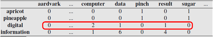
Note similarity of rows for information and digital, and of rows for apricot and pineapple.

Cosine similarity metric

$$ S(\mathbf v, \mathbf w) = \dfrac{\mathbf v^T \mathbf w}{\Vert\mathbf v\Vert \Vert\mathbf w\Vert} = \cos\theta $$

Exercise: compute cosine similarity between Apricot, Digital, and Information.

Term Frequency

1. TF: Frequent words more important than rare words. term frequency.

$$ tf(term,doc) = \begin{cases} 1+\log_{10} \text{Count}(term, doc), \text{ if } \text{Count}(term, doc)>0 \\ 0, \text{ else} \end{cases} $$

Log to dampen dominance of common words

plt.plot(np.linspace(1,10,100),1+ np.log(np.linspace(1,10,100)));

Inverse Document Frequency

1. Very frequent words very unimportant (a, and, the): inverse document frequency.

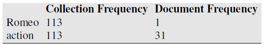
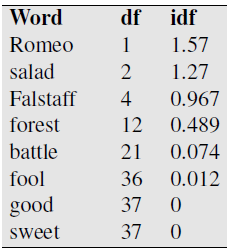
Document frequency $df(term)$ = # documents term appears in.

Collection frequency of term = # times term appears in collection.

Expect common words which are concentrated in fewer documents to be more discrimatory. Use inverse document frequency.

$$ idf(term) = \log_{10}\left(\dfrac{N}{df(term)}\right) $$

$N$ = total number of documents in collection

Words that appear in every document have low idf

tf-idf

tf-idf weighting is by far the dominant way of weighting co-occurrence matrices in information retrieval

$$ w(term, doc) = tf(term,doc) \times idf(term) $$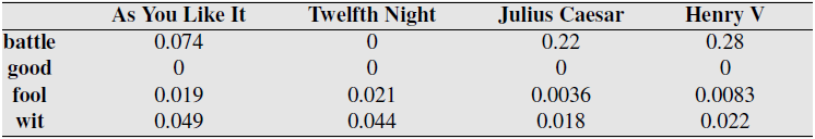

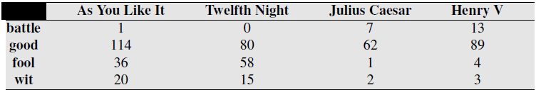
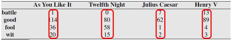
A tf-idf weighted term-document matrix for four words in four Shakespeare plays, using the counts in Fig. 6.2. Note that the idf weighting has eliminated the importance of the ubiquitous word good and vastly reduced the impact of the almost-ubiquitous word fool.

tf-idf Model

Compute word co-occurence matrix with counts weighted by tf-idf for word in document.

Represent words with vectors (rows or columns) from this matrix - tf-idf vectors.

Compare similarity between words using cosine metric of vectors.

Describe documents using average of tf-idf vectors for all contained words.

Pointwise Mutual Information (PMI)

Alternative weighting to tf-idf

Pointwise mutual information (Fano, 1961) is one of the most important concepts in NLP. It is a measure of how often two events x and y occur, compared with what we would expect if they were independent:

$$ PMI(x,y) = \log_2\left(\dfrac{P(x,y)}{P(x)P(y)}\right) = \log_2\left(\dfrac{\text{observed co-occurence}}{\text{co-occurence if independent}}\right) $$

where $x$ = target word, and $y$ = context word.

Positive Pointwise Mutual Information (PPMI)

$$ PMI(x,y) = \max\left\{ \log_2\left(\dfrac{P(x,y)}{P(x)P(y)}\right),0 \right\} $$

Eliminates all negative values which represent word occurring less often than random -- too rare to be reliable.

Dense Embeddings

Use short dense vectors rather than long sparse vectors

"It turns out that dense vectors work better in every NLP task than sparse vectors."

Possible reasons why:

• Easier to learn fewer parameters
• Less prone to overfitting
• May do a better job of capturing synonymy than sparse vectors

Example

In training data, 'car' and 'dashboard' are used together in sentence.

But in test data, 'dashboard' and 'automobile' are used together instead.

II. Dimensionality Reduction

Dimensionality Reduction - Motivation

1. Reducting problem complexity
   • Complexity of any classifier or regressor depends on the number of inputs.
   1. time and space complexity
   2. necessary number of training examples to train such a classifier or regressor.
   3. Curse of dimensionality
2. Visualization - 2D retina, 3D mental capacity, $n$-dimensional data

Feature selection - choose a subset of important features pruning the rest

Feature extraction - form fewer, new features from the original inputs

Main methods for dim reduction

1. Feature selection - given $d$ inputs, choose $k<d$ inputs to keep, discard the rest.
2. Feature extraction - compute $k<d$ new inputs using combinations of original inputs. E.g. replace multiple inputs with their average.

Feature extraction: Linear Methods

Here, linear means new features are linear combinations of original features. E.g. mean of multiple features.

• Principal Component Analysis (PCA) - use SVD & keep singular vectors for largest singular values

Exercise: write the SVD of your dataset and identify the combinations of original inputs

• Linear Discriminant Analysis (LDA) - supervised variation on PCA

• Factor Analysis -

• Multidimensional Scaling -

• Canonical correlation analysis - finds joint features that relate multiple datasets

Feature extraction: Nonlinear Methods

Here, nonlinear means new features are not linear combinations of original features. E.g. 2nd & higher order statistics (variance, correlation, skew)

Exercise: describe how to compute nonlinear statistical functions of features in dataset

• Isometric feature mapping

• Locally linear embedding

• Laplacian eigenmaps

Principal Component Analysis

1. Center the data

2. Rotate axes to line up directions of highest variance

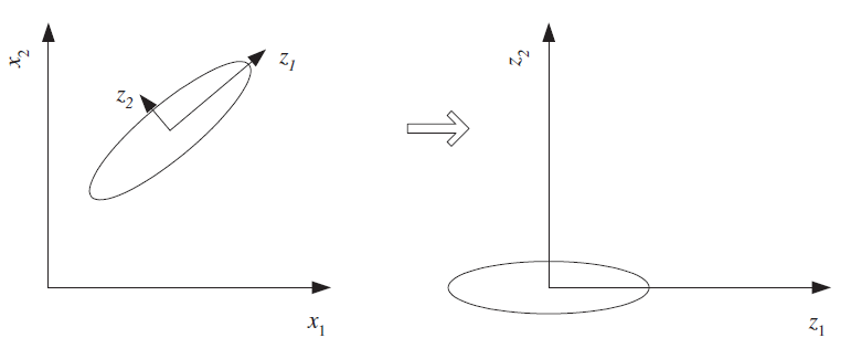
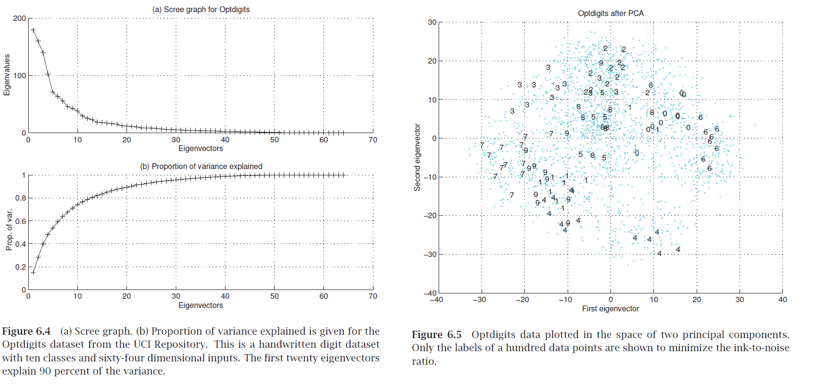
Scree graph

plot of variance explained as a function of the number of eigenvectors kept

Exercise: how do you compute "variance explained"?

"Eigendigits" = eigenvectors of handwritten digit image dataset (with images as rows).

Exercise 2: what are the original and extracted features in the geometric figure?

Feature Embedding

$\mathbf X$ is $N\times d$ data matrix.

"Centered to have zero mean" (row means)

$d\times d$ covariance matrix = $\mathbf X^T \mathbf X$

Eigenvector decomposition $\mathbf X^T \mathbf X = \mathbf W \mathbf D \mathbf W^T$

Truncate (length-$d$) eigenvectors $\mathbf w_i$ for $k$ largest eigenvalues.

Get coordinates of data point in eigenvector space by taking inner product of row $\mathbf x^{(j)}$ with eigenvectors $\mathbf w_i$. Note these are length-$n$ vectors.

Compute embedding coordinates in one shot: $\mathbf X \mathbf W = \mathbf F$ where columns of $\mathbf F$ are the embedded features.

Definition of our eigenvectors: $\mathbf X^T\mathbf X \mathbf W = \mathbf W\mathbf D$.

Multiply both sides by $\mathbf X$ to get $\mathbf X \mathbf X^T\mathbf X \mathbf W = \mathbf X \mathbf W\mathbf D$

Plug in definition of $\mathbf F$ to get $\mathbf X \mathbf X^T\mathbf F = \mathbf F \mathbf D$

We just proved that the embedding vectors (columns of $\mathbf F$) are eigenvectors of $\mathbf X \mathbf X^T$

Summary - two ways to compute embeddings of our data into eigenvector space:

1. Compute basis $\mathbf W$ as eigenvectors of $\mathbf X^T\mathbf X$, then project rows of $\mathbf X$ onto this basis (this is basically PCA)

2. Directly compute eigenvectors of $\mathbf X\mathbf X^T$.

Which way is more efficient?

"Embedding"?

Reconsider $\mathbf X \mathbf X^T$ matrix, elements are inner products between rows of $\mathbf X$ -- similarity measure between samples.

So we can view $\mathbf X \mathbf X^T$ as a weighted adjacency matrix of a graph relating the samples to each other.

By taking a truncated set of its eigenvectors we are doing graph embedding!

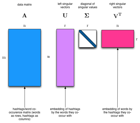
Singular Value Decomposition and Matrix Factorization

$$\mathbf X = \mathbf V \mathbf A \mathbf W^T$$

Columns of $\mathbf V$ are eigenvectors of $\mathbf X \mathbf X^T$

Columns of $\mathbf W$ are eigenvectors of $\mathbf W \mathbf W^T$

Diagonal of $\mathbf A$ contains singular values, squaare roots of eigenvalues of $\mathbf X \mathbf X^T$ and $\mathbf W \mathbf W^T$

Topic Modeling

• Determine small set of topics for corpus of documents, e.g. politics, art, sports
• Unsupervised learning problem - factor word-document matrix - SVD, NNMF, Latent Dirichlet Allocation

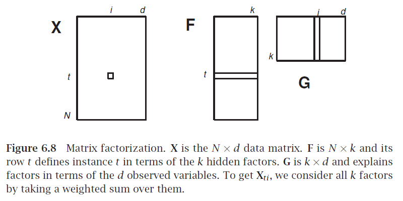
Matrix Factorization

Break matrix into two or more $\mathbf X = \mathbf F \mathbf G$

Analogous to factoring a number, e.g. $28 = 7 \times 2 \times 2$

If $\mathbf X$ is $N \times d$, what are sizes of factors?

$\mathbf G$ as factors in terms of original features

$\mathbf F$ as samples transformed to factor combinations

Latent Semantic Indexing

$\mathbf X$ is a sample of $N$ documents each using a bag of words representation with $d$ words

each factor may be one topic or concept written using a certain subset of words

each document is a certain combination of such factors

$\mathbf G$ relates documents to factors

$\mathbf F$ relates words to factors

Application: Recommender System

We have $N$ customers and we sell $d$ different products

$X_{ij}$ is number of times customer $i$ bought product $d$

$\mathbf G$ relates customers to factors

$\mathbf F$ relates products to factors

...point of these is to get some new customer or document and compute something...

Latent dirichlet allocation (LDA; Blei et al., 2003)

• one of the most widely used techniques in machine learning
• still the standard way to do topic modelling.

https://scikit-learn.org/stable/modules/generated/sklearn.decomposition.LatentDirichletAllocation.html

III. Word Embedding

Word embedding - Motivation

Most machine learning methods are based on numerical mathematical mathods which operate on vectors of numbers. E.g. deep learning.

But when text is converted to numbers via most common approaches, the numbers are not very meaningful.

Example of meaningful vectors:

• array of light levels in image
• list of concentration levels of chemicals

Example of less-meaningful vectors:

• list of base-pairs in DNA converted to 0,1,2,3
• list of ascii code of letters in document

Goal: Convert text into vectors who's geometric locations are meaningful. So similar text passages have similar vectors

Pretrained word embeddings

• used to initialize the first layer in models.
• do not require labeled data - vast amounts of unlabele data available
• use as embeddings, or fine tune on task

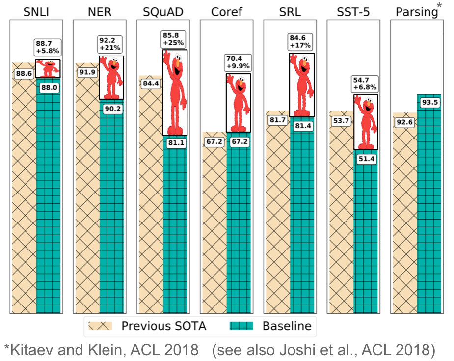
ELMo = Em-beddings from Language Models "a deep contextualized word representation that models both (1) complex characteristics of word use (e.g., syntax and semantics), and (2) how these uses vary across linguistic contexts (i.e., to model polysemy). These word vectors are learned functions of the internal states of a deep bidirectional language model (biLM), which is pre-trained on a large text corpus. They can be easily added to existing models and significantly improve the state of the art across a broad range of challenging NLP problems, including question answering, textual entailment and sentiment analysis."

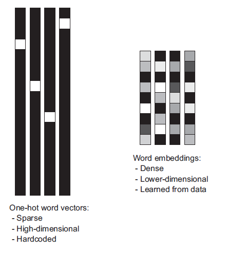
Word embeddings

One-hot encoding converts words (or $n$-grams) into orthogonal vectors $\mathbf e_k$ with a single "1" value and the rest zeros. Vectors for any two words are orthogonal. So to handle 50,000 words requires length-50,000 vectors.

Geometrically these are orthogonal vectors in 50,000-dimensional space. With every word vector equally-distant from every other.

Word embeddings try to squeeze these into a lower number of dimensions by putting "similar" words closer together, use real numbers (rather than only binary).

Word embedding - Approach

Use machine learning method which assigns vectors by learning similarity

Two-step process:

1. Convert text to numbers via simple approach
2. Dimensionality reduction

Q: Isn't embedding basically just another name for dimensionality reduction done for the usual reasons (to reduce need for data)?

A: Yes. But there's some new methods devised under this new name.

Embedding methods

• Principal component analysis & related methods applied to BOW data ~ Latent semantic indexing
• GloVe - Dim reduction on matrix of co-occurence statistics.
• Shallow neural network layer - Embedding layer
  • Neural embedding: word2vec, doc2vec, x2vec

Exercise - Embedding Layer

1. Draw a dense linear single-layer network with no activation function, with $N$ inputs and $m$ outputs,

2. write the output for a one-hot encoded input vector $\mathbf e_k$ representing a single word.

3. write the output for a general input vector $\mathbf v$ representing multiple words in a document.

Latent Semantic Indexing

Recall Matrix Factorization: Break matrix into two or more $\mathbf X = \mathbf F \mathbf G$

$\mathbf X$ is a sample of $N$ documents each using a bag of words representation with $d$ words

each factor may be one topic or concept written using a certain subset of words

each document is a certain combination of such factors

$\mathbf G$ relates documents to factors

$\mathbf F$ relates words to factors

GloVe - Global Vectors for Word Representation

Can download and use result: https://nlp.stanford.edu/projects/glove/

"Visualizing Embeddings"

Listing most-similar words for given word based on cosine distance

GloVe: 
    given word: frog 
    most similar words: frogs, toad, litoria, leptodactylidae, rana, lizard, and eleutherodactylus

Clustering words based on cosine distance - hierarchical representation

Project embedding space to 2D

Semantic Properties of Embeddings

context window size

• small window - semantically-similar words, same parts of speech
• large window - topically related words, not similar

First order co-occurence (syntagmatic association) - words typically near each other. $wrote$ and $book$

Second-order co-occurrence (paradigmatic association) - have similar neighbors $wrote$ and $said$

Relational meanings (analogous meanings) via word differences: $king-man+woman = queen$

• gender vector
• comparative & superlative morphology
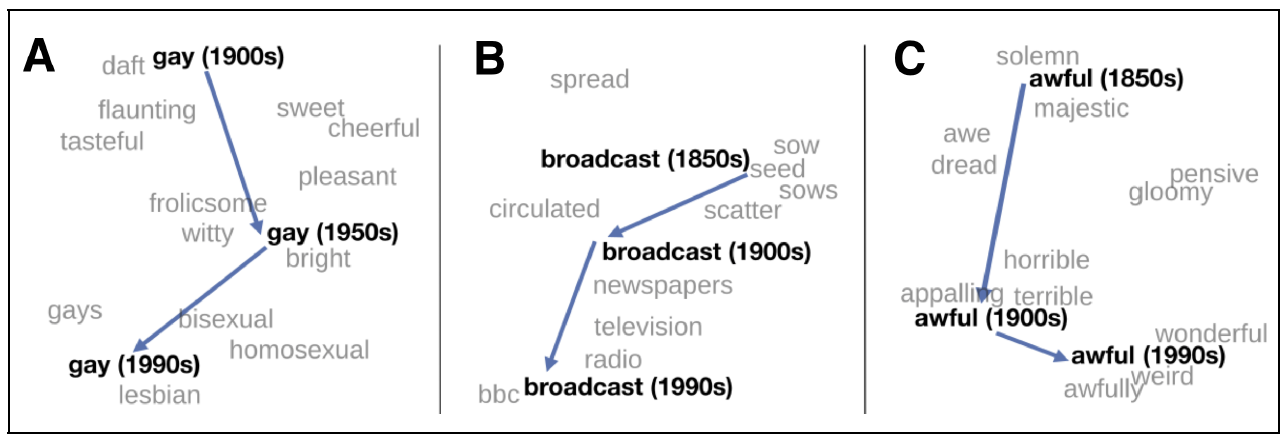
• temporal changes
• bias: $doctor-man+woman = nurse$

Evaluating embeddings

Compare embedded distance to human-estimated similarity

• WordSim-353 (Finkelstein et al., 2002) is a commonly used set of ratings from 0 to 10 for 353 noun pairs;
• SimLex-999 (Hill et al., 2015) quantifies similarity (cup, mug) rather than relatedness (cup, coffee), and including both concrete and abstract adjective, noun and verb pairs.
• TOEFL dataset (Landauer and Dumais, 1997) - 80 questions consisting of a target word with 4 additional word choices for closest synonym.
• Stanford Contextual Word Similarity (SCWS) dataset (Huang et al., 2012) - human judgments on 2,003 pairs of words in their sentential context, including nouns, verbs, and adjectives.
• semantic textual similarity task (Agirre et al. 2012, Agirre et al. 2015) evaluates the performance of sentence-level similarity algorithms, consisting of a set of pairs of sentences, each pair with human-labeled similarity scores
• Analogy task datasets (Mikolov et al. 2013, Mikolov et al. 2013b) a is to b as c is to d

Perplexity

Metric to compare language models

$$ PP(W) = \left( \prod_{i=1}^N \frac{1}{P(w_{i}|w_{i−1})} \right)^\frac{1}{N} $$