Unstructured Data & Natural Language Processing

Topic: Neural Language Modeling & Embedding

This topic:

1. Neural Language models
2. Neural word embedding
3. Beyond words

Reading:

• J&M Chapter 7 (Neural Networks and Neural Language Models)
• Young et al, "Recent trends in deep learning based natural language processing" 2018
• Sebastian Ruder, "A Review of the Neural History of Natural Language Processing" 2018

http://blog.aylien.com/a-review-of-the-recent-history-of-natural-language-processing/

• 2001 – Neural language models
• 2008 – Multi-task learning
• 2013 – Word embeddings
• 2013 – Neural networks for NLP
• 2014 – Sequence-to-sequence models
• 2015 – Memory-based networks
• 2018 – Pretrained language models

... 2016-2018 - Attention

... 2017 - Transformer networks

... 2019 - BERT

I. Neural Language models

Neural language models

"the task of predicting the next word in a text given the previous words"

• applications such as intelligent keyboards (predict incomplete word, next word) and email response suggestion (Kannan et al., 2016)

Classic approaches are based on n-grams and employ smoothing to deal with unseen n-grams (Kneser & Ney, 1995)

a form of unsupervised learning, also called predictive learning by Yann LeCun

"Sequence" model

$$P(\text{first word}=\text{"once"},\text{second word}=\text{"upon"},\text{third word}=\text{"a"},\text{fourth word}=\text{"time"})$$

Or with vector notation $P(\mathbf w)$, where $w_1$="once", $w_2$="upon", $w_3$="a", $w_4$="time".

Note these are not quite the same as the simple joint probability of the words, i.e.,

$$P(\text{"once"},\text{"upon"},\text{"a"},\text{"time"}) = P(\text{"upon"},\text{"a"},\text{"time"},\text{"once"}) = ...$$

Unless we choose to ignore relative location of words (will get to that soon).

"Predictive" model

$$P(\text{fourth word}=\text{"time"}\,|\,\text{first word}=\text{"once"},\text{second word}=\text{"upon"},\text{third word}=\text{"a"})$$

Different versions of same information. Both are referred to as "language models".

$N$-grams

Model order limited to length $N$ sequences:

\begin{align} P(w_n|w_{n-1}...w_1) &\approx P(w_n|w_{n-1}...w_{n-(N-1)}) \\ P(w_n|w^{n-1}_1) &\approx P(w_n|w^{n-1}_{n-N+1}) \end{align}

So use previous $N-1$ words.

1. Unigram
2. Bigram
3. Trigram

Formal Machine Learning Framework & Jargon

1. Given training data $(\mathbf x_{(i)},y_i)$ for $i=1,...,m$.

2. Choose a model $f(\cdot)$ where we want to make $f(\mathbf x_{(i)})\approx y_i$ (for all $i$)

3. Define a loss function $L(f(\mathbf x), y)$ to minimize by changing $f(\cdot)$ ...by adjusting the weights.

Machine Learning Framework using Sklearn

1. Given training data $(\mathbf x_{(i)},y_i)$ for $i=1,...,m$ --> lists of samples $\verb|X|$ and labels $\verb|y|$

2. Choose a model $f(\cdot)$ where we want to make $f(\mathbf x_{(i)})\approx y_i$ (for all $i$) --> choose sklearn estimator to use

3. Define a loss function $L(f(\mathbf x), y)$ to minimize by changing $f(\cdot)$ ...by adjusting the weights --> default choices for estimators, sometimes multiple options

class Estimator(object):
  
    def fit(self, X, y=None):
        """Fit model to data X (and y)"""
        self.some_attribute = self.some_fitting_method(X, y)
        return self
            
    def predict(self, X_test):
        """Make prediction based on passed features"""
        pred = self.make_prediction(X_test)
        return pred
    
model = Estimator()

Deep Learning

In addition to usual Machine Learning process - we perform the art of utilizing an artificial neural network

1. Make up an architecture - choose layers and their parameters - define custom $f(\mathbf x_{(i)})$

2. Choose a Loss function - how compute error for $f(\mathbf x_{(i)}) \ne y_i$

3. Choose a optimization method - many variants of same basic method

4. Choose "regularization" tricks to prevent overfitting

5. Handle other important details like initializing and normalizing data

Exercise

1. Given training data $(\mathbf x_{(i)},y_i)$ for $i=1,...,m$.

2. Choose a model $f(\cdot)$ where we want to make $f(\mathbf x_{(i)})\approx y_i$ (for all $i$)

3. Define a loss function $L(f(\mathbf x), y)$ to minimize by changing $f(\cdot)$ ...by adjusting the weights.

How might we apply this to language models?

What is $(\mathbf x_{(i)},y_i)$?

What is $L(f(\mathbf x), y)$?

How might you use your model to accomplish something useful?

Neural Language models

1. Feedforward neural language models - Bengio et al (2003), J&M Ch. 7
2. Recurrent neural language models - most modern neural language models (coming up)

Feedforward neural language model (Bengio et al. 2003)

Estimate probability of word given previous $N$ words, analogous to $N$-gram

$$ P(w_t|w_1^{t-1}) \approx P(w_t|w_{t-N+1}^{t-1}) $$

However neural language models relate Embeddings of words rather than exact words

Universal Function approximation

• A sufficiently complex neural network can model any function $f(\mathbf x) = \mathbf y$ given sufficient training data
• View language model $P(w_t|w_1^{t-1})$ as a function to model

Neural language model

The first neural language model, a feed-forward neural network proposed in 2001 by Bengio et al:

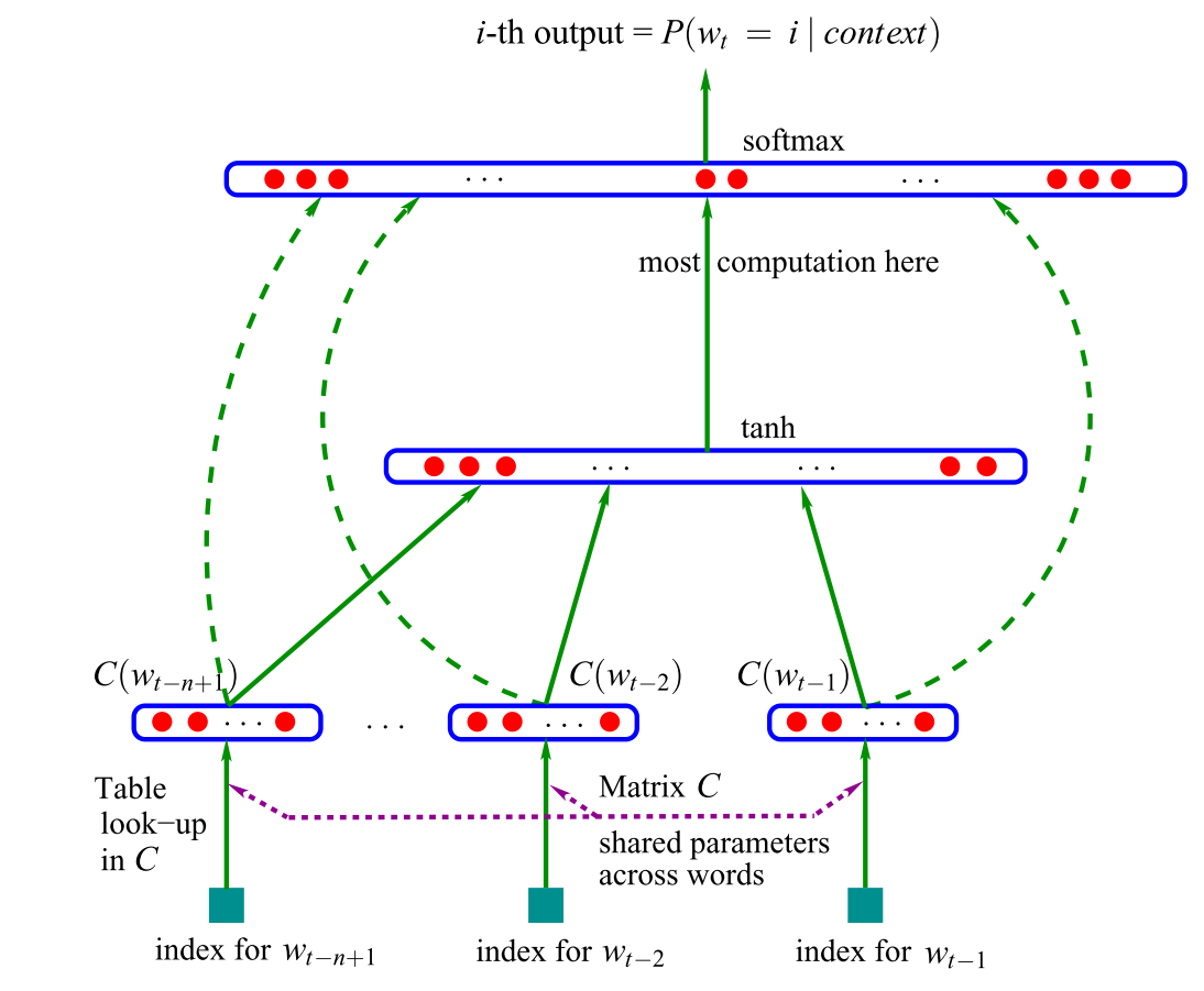
1. input = vector representations of the n previous words, which are looked up in a table C. A.k.a. word embedding layer
2. the word embeddings are concatenated and fed into a hidden layer,
3. hidden layer output is then provided to a softmax layer

How do you perform table lookup with matrix multiplication?

How do you implement vector-matrix multiplication with a neural network?

A softmax output layer is key to the network producing a language model. Why?

Extensions and more recent language models

• recurrent neural networks (Mikolov et al., 2010)

• long short-term memory networks (Graves, 2013)

• Word embeddings: basically an initial layer that does dimensionality reduction, very widely used perspective.

• Sequence-to-sequence models generate an output sequence by predicting one word at a time.

• Pretrained language models use representations from language models for transfer learning.

II. Neural Word Embeddings

Recap

Bag-of-words model - a sparse vector representations of text

Word embedding - a linear stage which converts sparse input into dense vector representations of words

1. Bengio et al 2001 - an initial linear layer in the Neural Language Model
2. Collobert & Weston 2008 - sharing of embedding layers between networks performing different NLP tasks

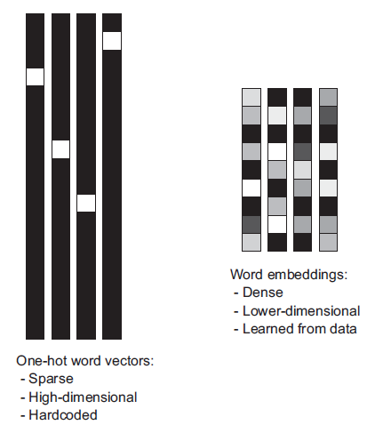
Word embeddings

One-hot encoding converts words (or $n$-grams) into orthogonal vectors $\mathbf e_k$ with a single "1" value and the rest zeros. Vectors for any two words are orthogonal. So to handle 50,000 words requires length-50,000 vectors.

Geometrically these are orthogonal vectors in 50,000-dimensional space. With every word vector equally-distant from every other.

Word embeddings try to squeeze these into a lower number of dimensions by putting "similar" words closer together, use real numbers (rather than only binary).

Embedding matrix $\mathbf E$

• $V$ rows, one for each word
• Each row is $d$-dimensional embedding vector

Multiply $\mathbf E^T$ by one-hot encoded word to get word embedding

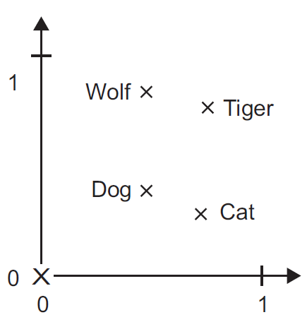
Test for understanding

Suppose

1. these four words are our entire vocabulary.
2. these points are the embeddings.

What is the embedding matrix for this situation?

Word2Vec embedding

Mikolov et al 2013

Basically simplified version of neural language model

• more efficient - scalable to very large dataset
• main goal is to produce embedding weights to re-use elsewhere
• use of such "pre-trained" embeddings shown to improve performance in other networks/tasks.

The intuitive geometric relations between vectors representing words attracted a great deal of interest

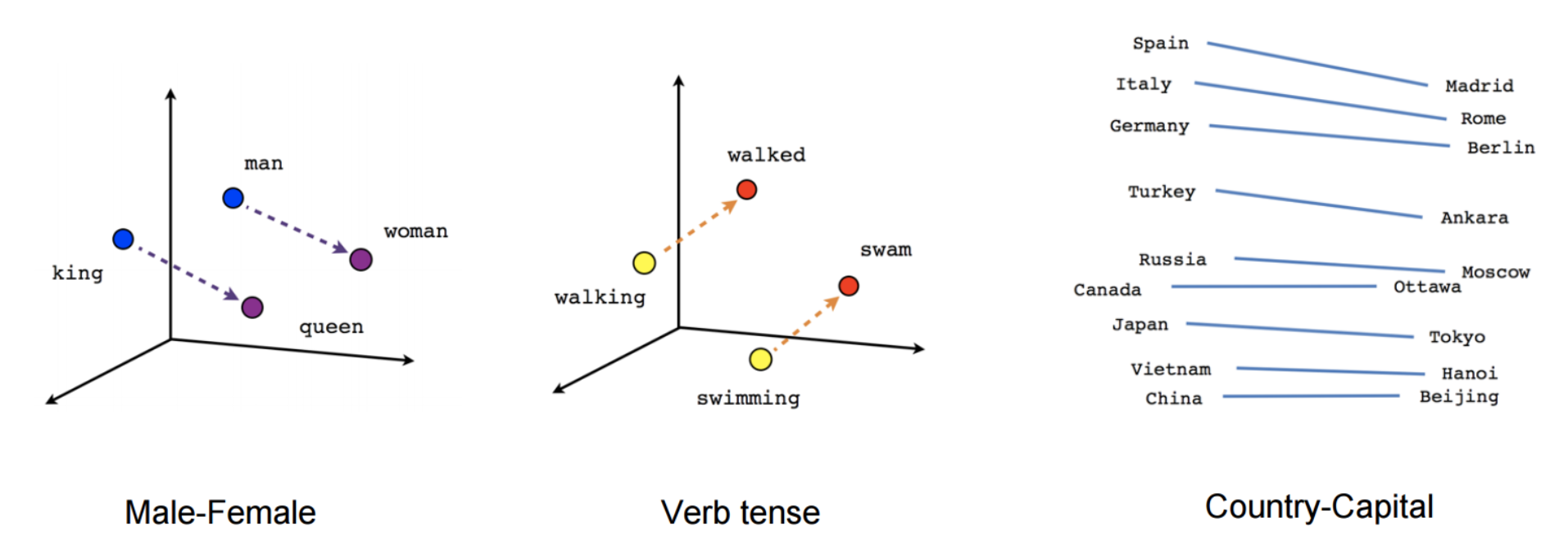
word2vec general idea: model probability of both target word with context.

“Is word w likely to show up near apricot?”

Use running text as implicitly supervised training data

• no need for hand-labeling
• Bengio 2003 and Collobert 2011 used for neural language model

word2vec = Simplified case of neural language model

1. Binary classifier - learn to identify neighboring word versus randomly-chosen word ("noise word").
2. Logistic regression - then use regression weights as embeddings.

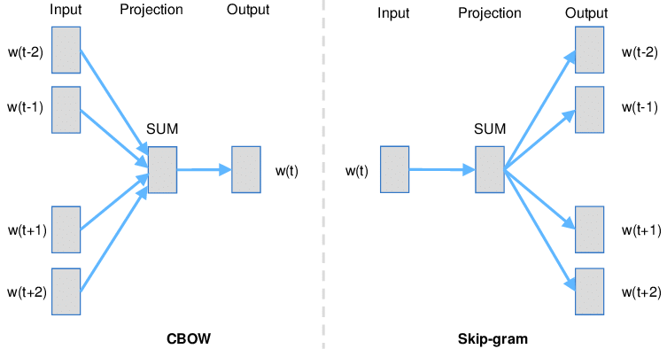
word2vec contains two algorithms:

1. Continuous Skip-gram - predict neighboring words of given word
2. Continuous bag-of-words (CBOW) - predict target word given neighbors

Continuous = dense embedding vector rather than sparse binary.

Negative Sampling = minimize the log-likelihood of those randomly-chosen other words from lexicon. "Skip-gram with Negative Sampling (SGNS)"

1. Continuous bag of words (CBOW) - predict $k$th word using neighbors in a window
2. Skip-gram - predict neighboring words for $k$th word

The weights in the neural layer for prediction give the emedding matrix.

Can download and use result: https://code.google.com/archive/p/word2vec

The classifier

Given tuple of words $(t,c)$, e.g. $(apricot,jam)$:

• $t$ = target word
• $c$ = candidate context word

Predict $P(+|t,c)$ probability $c$ is a context word.

Probability $c$ is not a context word: $P(-|t,c) = 1- P(+|t,c)$

Classifier model - basically just a similarity metric, made into probability by sigmoid function.

\begin{align} P(+|t,c) &= \sigma(\text{"similarity"}) \\ &= \frac{1}{1-e^{-\mathbf t \cdot \mathbf c}} \end{align}

where $\mathbf t$ and $\mathbf c$ are the dense vectors representing the words -- these are the parameters of the model which we will fit using data.

\begin{align} P(-|t,c) &= 1-P(+|t,c) \\ &= \frac{e^{-\mathbf t \cdot \mathbf c}}{1-e^{-\mathbf t \cdot \mathbf c}} \end{align}

"skip-gram"

A variation on a bigram which combines target word and context word (not necessarily neighbor), hence it "skips" other context words.

Context words assumed independent of each other, so for a target word and list of context words,

\begin{align} P(+|t,(c_1, c_2,...)) &= \prod_i \frac{1}{1-e^{-\mathbf t \cdot \mathbf c_i}} \end{align}

Bigrams:

• $t$ and immediately preceding word
• $t$ and immediately following word

Skip-grams:

• $t$ and word two words away
• $t$ and word three words away
• ...

Examples:

Hyperparameter: ratio between numbers of positive and negative examples $k$ (=2 above)

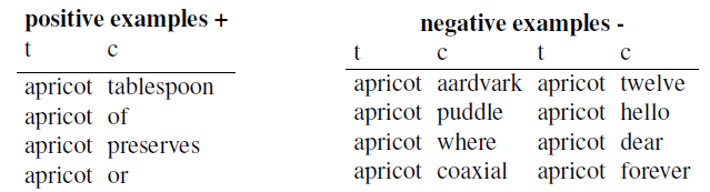
Noise word choice

Sampled from lexicon according to weighted unigram frequency $P_\alpha(w)$

$$P_\alpha(w) = \frac{[C(w)]^\alpha}{\sum_{w'} [C(w')]^\alpha }$$

$\alpha = 0$: ignore unigram probability altogether. Use rare words and common words equally often.

$\alpha<1$: dampen high probabilities (like for $w=the$). Use common words more, but not as much more as their frequency in lexicon.

Common choice: $\alpha = 0.75$

Optimization of model

Start by making training set $D$ of skip grams $(t_i, c_i)$ with target words and context words.

Note that if we simply try to maximize $\prod_i P(+|t,c_i) = \prod_i \dfrac{1}{1-e^{-\mathbf t_i \cdot \mathbf c_i}}$ by choosing $\mathbf t_i$ and $\mathbf c_i$, we can get an optimal by making all $\mathbf t_i = \mathbf t_j = \mathbf c_i = \mathbf c_j$.

Hence we also need a term in our optimization objective to force the vectors apart and counter this useless trivial solution. This is the negative samples.

So we augment the training set with a negative set $D'$ with fake skip grams $(t_j,c'_j)$ using noise words for the $c'_j$.

Then try to maximize $\prod_i P(+|t_i,c_i) \prod_j P(-|t'_j,c'_j)$.

In other words we want a model which has high probabilities for all the skip grams in the set $D$, and another model with high probabilities for all the negative samples in the set $D'$.

Taking the log of the objective we get

\begin{align} &\max_{\mathbf t_k,\mathbf c_k} \sum_{(t_i,c_i)\in D} \log \frac{1}{1-e^{-\mathbf t_i \cdot \mathbf c_i}} + \sum_{(t_j,c_j)\in D'} \log \frac{e^{-\mathbf t_j \cdot \mathbf c_j}}{1-e^{-\mathbf t_j \cdot \mathbf c_j}} \end{align}

Note that the parameters are two sets of vectors, the $\mathbf t_k$ and $\mathbf c_k$ which we can form into matrices $\mathbf T$ and $\mathbf C$.

The result is two different embedding vectors for each word, one when it is target and one when it is context. We can just choose one or combine them (e.g. take average).

Hyperparameters

• $k$ - the ratio of negative samples to context samples
• $\alpha$ - the weighting for negative sampling
• $L$ - the context window size

III. Embedding Uses

Multi-task Learning

• Caruana, 1998 - road-following + pneumonia prediction
• Train models to learn representations that are useful for many tasks.
• For learning general, low-level representations, for settings with limited amounts of training data

Multi-task Learning - Sharing of initial layer weights, a.k.a. word embedding matrices

Collobert & Weston, 2008; Collobert et al., 2011

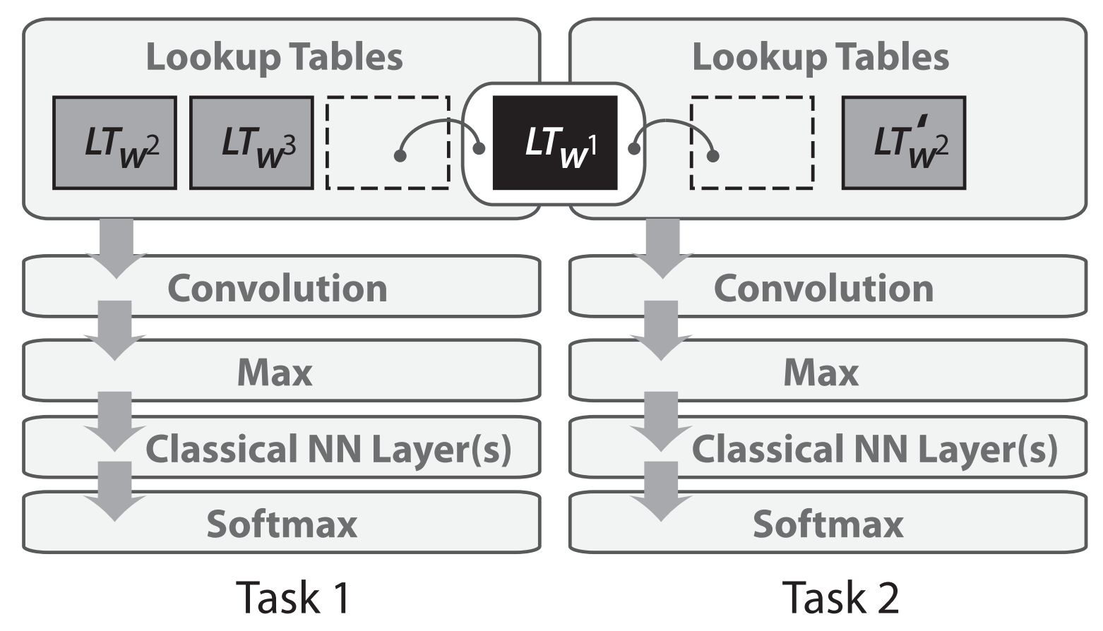
• word embedding matrices are shared between two models trained on different tasks
• paper also suggested pretraining word embeddings
• and using convolutional neural networks (CNNs) for text

Neural Translation with embeddings - Cross-lingual transfer

zero-shot cross-lingual transfer - project word embeddings of different languages into the same space

Unsupervised learning methods

Using non-neural embeddings in neural network

• Nothing inherently special about word2vec
• Word embeddings can also be learned via matrix factorization (Pennington et al, 2014; Levy & Goldberg, 2014)
• Even SVD and LSA have been shown to achieve similar results (Levy et al., 2015)
• word2vec is still a popular choice and widely used

GloVe

Pennington et al, 2014

Dim reduction on matrix of co-occurence statistics.

Can download and use result: https://nlp.stanford.edu/projects/glove/

glove_dir = '/home/user01/Public/Data/Glove_embeddings'

embeddings_index = {}
f = open(os.path.join(glove_dir, 'glove.6B.100d.txt'))
for line in f:
    values = line.split()
    word = values[0]
    coefs = np.asarray(values[1:], dtype='float32')
    embeddings_index[word] = coefs
f.close()

print('Found %s word vectors.' % len(embeddings_index))

Found 400000 word vectors.

# make embedding matrix

embedding_dim = 100

embedding_matrix = np.zeros((max_words, embedding_dim))
for word, i in word_index.items():
    embedding_vector = embeddings_index.get(word)
    if i < max_words:
        if embedding_vector is not None:
            # Words not found in embedding index will be all-zeros.
            embedding_matrix[i] = embedding_vector

embedding_matrix.shape

(10000, 100)

Keras Embedding Layer

Literally download GloVe or word2vec and use .set_weights() to set it as weights

See Chollet Ch.6 for examples

from keras.models import Sequential
from keras.layers import Embedding, Flatten, Dense

model = Sequential()
model.add(Embedding(max_words, embedding_dim, input_length=maxlen))
model.add(Flatten())
model.add(Dense(32, activation='relu'))
model.add(Dense(1, activation='sigmoid'))
model.summary()

_________________________________________________________________
Layer (type)                 Output Shape              Param #   
=================================================================
embedding_2 (Embedding)      (None, 100, 100)          1000000   
_________________________________________________________________
flatten_1 (Flatten)          (None, 10000)             0         
_________________________________________________________________
dense_1 (Dense)              (None, 32)                320032    
_________________________________________________________________
dense_2 (Dense)              (None, 1)                 33        
=================================================================
Total params: 1,320,065
Trainable params: 1,320,065
Non-trainable params: 0
_________________________________________________________________

# Set embedding layer weights to GloVe matrix and freeze

model.layers[0].set_weights([embedding_matrix])
model.layers[0].trainable = False

Beyond words

• Representations for sentences Mikolov & Le, 2014
• Skip-Thought Vectors (sentence representations) - Kiros et al., 2015
• nodevec - Modeling networks (Grover & Leskovec, 2016)
• Modeling biological sequences (Asgari & Mofrad, 2015)

Lab

Download embedding weights and compute cosine distances between similar words.