Unstructured Data & Natural Language Processing
Topic: Intro to Neural Networks with Keras
Today:
- Background: from Language models to machine learning
- Keras
- Keras Demo
- Convolutional Neural Networks
Reading:
- Chollet Chapter 3 (Getting started with neural networks)
- Chollet Chapter 6 (Deep learning for text and sequences)
- Geron, 2e Chapter 10 (Introduction to Artificial Neural Networks with Keras)
- "Text classification with preprocessed text: Movie reviews" https://www.tensorflow.org/tutorials/keras/text_classification
- "Getting Started with TensorFlow and Deep Learning: SciPy 2018 Tutorial", Josh Gordon, https://www.youtube.com/watch?v=tYYVSEHq-io
I. Background
Language models
"Sequence" model
$$P(\text{first word}=\text{"once"},\text{second word}=\text{"upon"},\text{third word}=\text{"a"},\text{fourth word}=\text{"time"})$$"Predictive" model
$$P(\text{fourth word}=\text{"time"}\,|\,\text{first word}=\text{"once"},\text{second word}=\text{"upon"},\text{third word}=\text{"a"})$$Different versions of same information. Both are referred to as "language models".
$N$-grams
Model order limited to length $N$ sequences:
\begin{align} P(w_n|w_{1}...w_{n-1}) &\approx P(w_n|w_{n-(N-1)}...w_{n-1}) \\ P(w_n|w^{n-1}_1) &\approx P(w_n|w^{n-1}_{n-N+1}) \end{align}- Unigram
- Bigram
- Trigram
Use previous $N-1$ words, relative frequencies of $N$-grams to estimate probabilities.
This is not machine learning, just statistics.
Applications of language models
- Spelling/Grammmar checking
- Word completion
- Autoregressive text generation
Word Embeddings
- many approaches
- simplest: dimensionality reduction of word-document marix
- reduce dimensions of words from thousands to hundreds
- new reduced dimensions are linear combination over words
Machine Learning: fitting functions (models) to data
$\bf x$ - input data ~ a single image, or sentence of text.
$\bf y$ - prediction ~ "cat" vs "dog", "positive" vs "negative"
$f(\cdot)$ - mapping from input to output - function we fit
Formal Machine Learning Framework & Jargon
Given training data $(\mathbf x_{(i)},y_i)$ for $i=1,...,m$.
Choose a model $f(\cdot)$ where we want to make $f(\mathbf x_{(i)})\approx y_i$ (for all $i$)
Define a loss function $L(f(\mathbf x), y)$ to minimize by changing $f(\cdot)$ ...by adjusting the weights.
Language model: $P(w_n|w_{1}...w_{n-1}) = f(\mathbf x_{(i)})\approx y_i$, so $w_{1}...w_n$ is $\mathbf x_{(i)}$, and $P \in [0,1]$ is $y$
Naive Bayes Classifier $c = \max_c P(c|w_{1}...w_{n}) = f(\mathbf x_{(i)})\approx y_i$, so $w_{1}...w_{n}$ is $\mathbf x_{(i)}$ and class $c \in \{0,1\}$ is $y$
Machine Learning Framework using Sklearn
Given training data $(\mathbf x_{(i)},y_i)$ for $i=1,...,m$ --> lists of samples $\verb|X|$ and labels $\verb|y|$
Choose a model $f(\cdot)$ where we want to make $f(\mathbf x_{(i)})\approx y_i$ (for all $i$) --> choose sklearn estimator to use
Define a loss function $L(f(\mathbf x), y)$ to minimize by changing $f(\cdot)$ ...by adjusting the weights --> default choices for estimators, sometimes multiple options
class Estimator(object):

    def fit(self, X, y=None):
        """Fit model to data X (and y)"""
        self.some_attribute = self.some_fitting_method(X, y)
        return self

    def predict(self, X_test):
        """Make prediction based on passed features"""
        pred = self.make_prediction(X_test)
        return pred

model = Estimator()
Deep Learning
Very flexible machine learning methods(s). I.e. there are many new options and variations to choose
Make up an architecture - choose layers and their parameters - define custom $f(\mathbf x_{(i)})$
Choose a Loss function - how compute error for $f(\mathbf x_{(i)}) \ne y_i$
Choose a optimization method - many variants of same basic method
Choose "regularization" tricks to prevent overfitting
Handle other important details like initializing and normalizing data
Multilayer (Artificial) Neural Networks - "Feed forward"
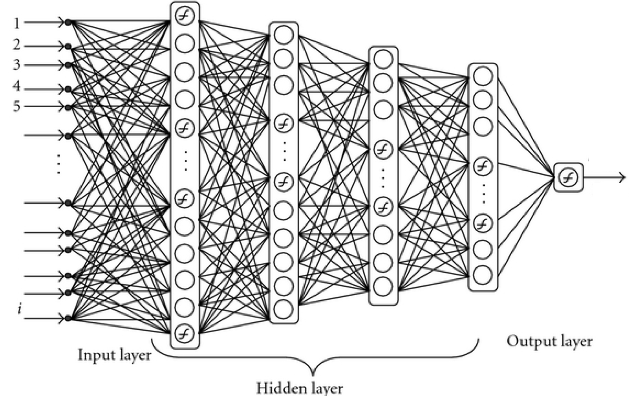
This is just a big complex model that computes $y = f(\mathbf x)$
Fundamental unit: artificial neuron
- input of some size
- weights
- Activation function
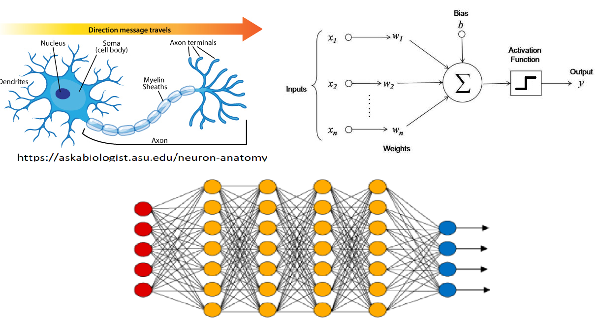
Operation
- computes a weighted sum of its inputs $z = w_1 x_1 + w_2 x_2 + ... + w_n x_n + b= \mathbf w^T \mathbf x +b$,
- then applies a step function to that sum and outputs the result: $h_{\mathbf w}(\mathbf x) = \sigma(z) = \sigma(\mathbf w^T \mathbf x +b)$
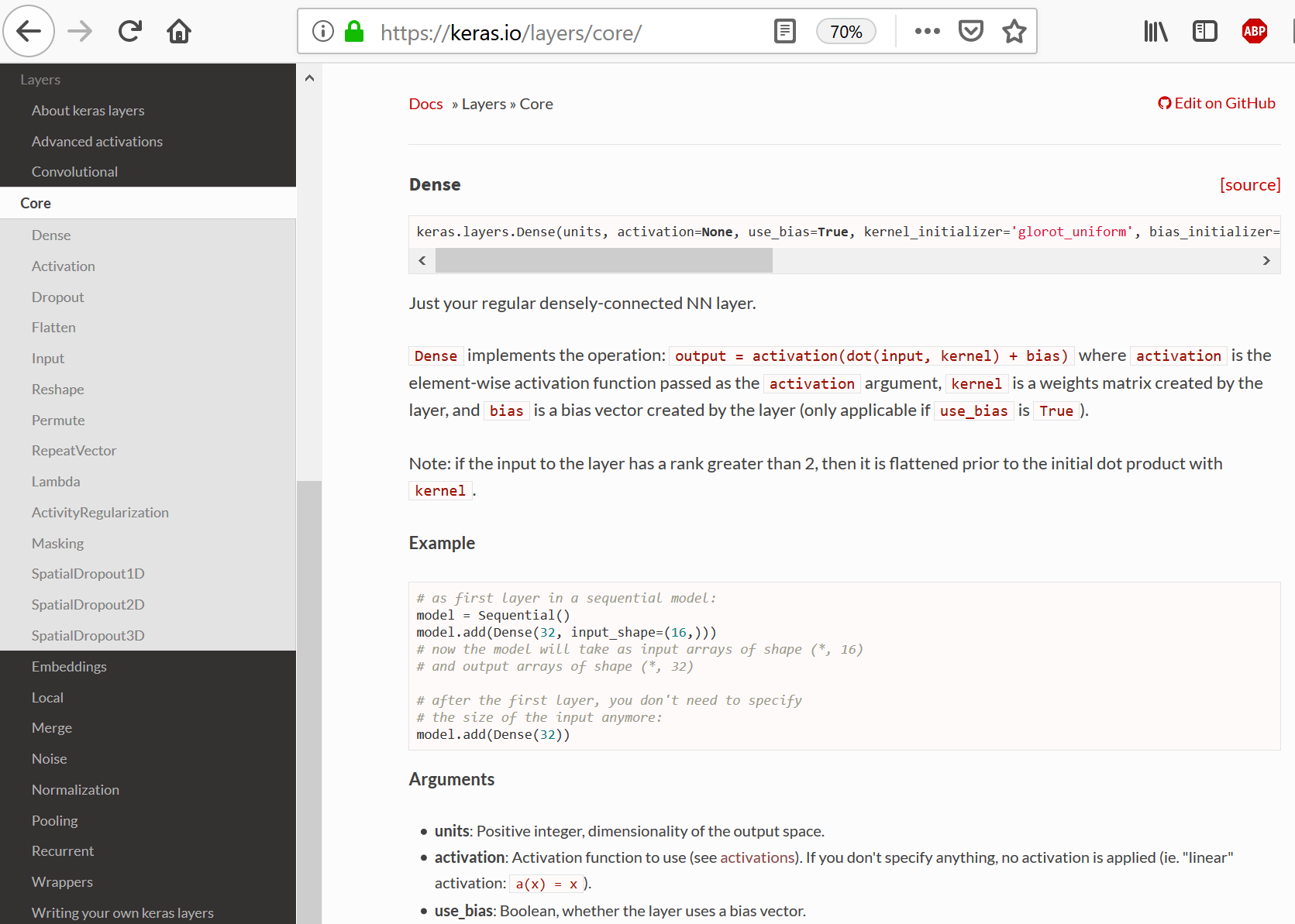
II. Keras

Fully-connected Layer
a.k.a. Densely-connected Layer - every input connects to every output (with weights)
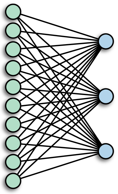
- Each node computes a weighted sum of all inputs $z_i = w_1 x_1 + w_2 x_2 + ... + w_n x_n + b_i= \mathbf w_i^T \mathbf x + \mathbf b$,
- Then applies a step function to that sum and outputs the result: $\mathbf h(\mathbf x) = \sigma(\mathbf z) = \sigma(\mathbf W^T \mathbf x + \mathbf b)$
Layers in Keras
Connection decisions: Fully-connected Layers, Convolutional Layers
Unified way to define other aspects of network: activation function, dropout, even pre-processing steps
Deep Network Design
Make up an architecture - choose layers and their parameters
Choose a Loss function - how compute error for $f(\mathbf x_{(i)}) \ne y_i$
Choose a optimization method - many variants of same basic method
Choose "regularization" tricks to prevent overfitting
Other important details like initializing and normalizing data
Keras Embedding Layer
Literally download GloVe or word2vec and use .set_weights() to set it as weights
$$\mathbf h(\mathbf x) = \sigma(\mathbf z) = \sigma(\mathbf W^T \mathbf x + \mathbf b) = \mathbf E^T \mathbf x$$See Chollet Ch.6 for examples
from keras.models import Sequential
from keras.layers import Embedding, Flatten, Dense

model = Sequential()
model.add(Embedding(max_words, embedding_dim, input_length=maxlen))
model.add(Flatten())
model.add(Dense(32, activation='relu'))
model.add(Dense(1, activation='sigmoid'))
model.summary()
# Set embedding layer weights to GloVe matrix and freeze

model.layers[0].set_weights([embedding_matrix])
model.layers[0].trainable = False
Using a (fixed-length) sequence of words as inputs
Notice output shape was 3D, because each sample consisted of a list of words, each embedded to a vector
For each word in an input consisting of $$\mathbf h(\mathbf x) = \sigma(\mathbf z) = \sigma(\mathbf W^T \mathbf x + \mathbf b) = [\mathbf E^T \mathbf x^{(1)},\mathbf E^T \mathbf x^{(2)},...,\mathbf E^T \mathbf x^{(N)}]$$
"Flatten" layer converted this to a single concatenated vector
III. Keras Demo
Shallow network (logistic regression) IMDB demo
Tensorflow demo (with Keras): Text classification with preprocessed text - Movie reviews https://www.tensorflow.org/tutorials/keras/text_classification
Chollet has a similar model and notebook which attempts to use GloVe embeddings. Unfortunately it doesn't work.
Many more examples for Keras independently https://github.com/keras-team/keras/tree/master/examples
- $\mathbf x_i$ (samples) are encoded sequences (reviews)
- $y_i$ (targets) are review class (positive or negative)
- Goal is to train model to predict review from text
Imports
install tensorflow-datasets via conda
import numpy as np
import tensorflow as tf
import tensorflow_datasets as tfds

print("Version: ", tf.__version__)
print("Eager mode: ", tf.executing_eagerly())
IMDB dataset
- Has been "encoded" so that the reviews (sequences of words) have been converted to sequences of integers
- Each integer represents a specific word in a dictionary.
To encode your own text see the Loading text tutorial
(train_data, test_data), info = tfds.load(
    'imdb_reviews/subwords8k', # Use the version pre-encoded with an ~8k vocabulary.
    split = (tfds.Split.TRAIN, tfds.Split.TEST), # Return the train/test datasets as a tuple.
    as_supervised=True, # Return (example, label) pairs from the dataset (instead of a dictionary).
    with_info=True) # Also return the `info` structure.
info
Encoder
The dataset info includes the text encoder (a tfds.features.text.SubwordTextEncoder).
encoder = info.features['text'].encoder
print ('Vocabulary size: {}'.format(encoder.vocab_size))
This text encoder will reversibly encode any string:
sample_string = 'Hello TensorFlow.'

encoded_string = encoder.encode(sample_string)
print ('Encoded string is {}'.format(encoded_string))

original_string = encoder.decode(encoded_string)
print ('The original string: "{}"'.format(original_string))

assert original_string == sample_string
The encoder encodes the string by breaking it into subwords or characters if the word is not in its dictionary. So the more a string resembles the dataset, the shorter the encoded representation will be.
for ts in encoded_string:
  print ('{} ----> {}'.format(ts, encoder.decode([ts])))
Explore the data
- The dataset comes preprocessed: each example is an array of integers representing the words of the movie review.
- The text of reviews have been converted to integers, where each integer represents a specific word-piece in the dictionary.
- Each label is an integer value of either 0 or 1, where 0 is a negative review, and 1 is a positive review.
for train_example, train_label in train_data.take(1):
  print('Encoded text:', train_example[:10].numpy())
  print('Label:', train_label.numpy())
The info structure contains the encoder/decoder. The encoder can be used to recover the original text:
encoder.decode(train_example)
Prepare the data for training
Create batches of training data for your model. The reviews are all different lengths, so use padded_batch to zero pad the sequences while batching
As of TensorFlow 2.2 the padded_shapes argument is no longer required. The default behavior is to pad all axes to the longest in the batch.
BUFFER_SIZE = 1000

train_batches = (
    train_data
    .shuffle(BUFFER_SIZE)
    .padded_batch(32, padded_shapes=([None],[])))

test_batches = (
    test_data
    .padded_batch(32, padded_shapes=([None],[])))
Each batch will have a shape of (batch_size, sequence_length) because the padding is dynamic each batch will have a different length:
for example_batch, label_batch in train_batches.take(2):
  print("Batch shape:", example_batch.shape)
  print("label shape:", label_batch.shape)
Build the model
The neural network is created by stacking layers—this requires two main architectural decisions:
- How many layers to use in the model?
- How many hidden units to use for each layer?
In this example, the input data consists of an array of word-indices. The labels to predict are either 0 or 1. Let's build a "Continuous bag of words" style model for this problem:
Caution: This model doesn't use masking, so the zero-padding is used as part of the input, so the padding length may affect the output. To fix this, see the masking and padding guide.
model = tf.keras.Sequential([
  tf.keras.layers.Embedding(encoder.vocab_size, 16),
  tf.keras.layers.GlobalAveragePooling1D(),
  tf.keras.layers.Dense(1)])

model.summary()
The layers are stacked sequentially to build the classifier:
- The first layer is an
Embeddinglayer. This layer takes the integer-encoded vocabulary and looks up the embedding vector for each word-index. These vectors are learned as the model trains. The vectors add a dimension to the output array. The resulting dimensions are:(batch, sequence, embedding). - Next, a
GlobalAveragePooling1Dlayer returns a fixed-length output vector for each example by averaging over the sequence dimension. This allows the model to handle input of variable length, in the simplest way possible. - This fixed-length output vector is piped through a fully-connected (
Dense) layer with 16 hidden units. - The last layer is densely connected with a single output node. Using the
sigmoidactivation function, this value is a float between 0 and 1, representing a probability, or confidence level. For numerical stability, use thelinearactivation function that represents the logits.
Hidden units
The above model has two intermediate or "hidden" layers, between the input and output. The number of outputs (units, nodes, or neurons) is the dimension of the representational space for the layer. In other words, the amount of freedom the network is allowed when learning an internal representation.
If a model has more hidden units (a higher-dimensional representation space), and/or more layers, then the network can learn more complex representations. However, it makes the network more computationally expensive and may lead to learning unwanted patterns—patterns that improve performance on training data but not on the test data. This is called overfitting, and we'll explore it later.
Loss function and optimizer
A model needs a loss function and an optimizer for training. Since this is a binary classification problem and the model outputs a probability (a single-unit layer with a sigmoid activation), we'll use the binary_crossentropy loss function.
This isn't the only choice for a loss function, you could, for instance, choose mean_squared_error. But, generally, binary_crossentropy is better for dealing with probabilities—it measures the "distance" between probability distributions, or in our case, between the ground-truth distribution and the predictions.
Later, when we are exploring regression problems (say, to predict the price of a house), we will see how to use another loss function called mean squared error.
Now, configure the model to use an optimizer and a loss function:
model.compile(optimizer='adam',
              loss=tf.losses.BinaryCrossentropy(from_logits=True),
              metrics=['accuracy'])
Train the model
Train the model by passing the Dataset object to the model's fit function. Set the number of epochs.
history = model.fit(train_batches,
                    epochs=10,
                    validation_data=test_batches,
                    validation_steps=30)
Evaluate the model
And let's see how the model performs. Two values will be returned. Loss (a number which represents our error, lower values are better), and accuracy.
loss, accuracy = model.evaluate(test_batches)

print("Loss: ", loss)
print("Accuracy: ", accuracy)
This fairly naive approach achieves an accuracy of about 87%. With more advanced approaches, the model should get closer to 95%.
Create a graph of accuracy and loss over time
model.fit() returns a History object that contains a dictionary with everything that happened during training:
history_dict = history.history
history_dict.keys()
There are four entries: one for each monitored metric during training and validation. We can use these to plot the training and validation loss for comparison, as well as the training and validation accuracy:
import matplotlib.pyplot as plt

acc = history_dict['accuracy']
val_acc = history_dict['val_accuracy']
loss = history_dict['loss']
val_loss = history_dict['val_loss']

epochs = range(1, len(acc) + 1)

# "bo" is for "blue dot"
plt.plot(epochs, loss, 'bo', label='Training loss')
# b is for "solid blue line"
plt.plot(epochs, val_loss, 'b', label='Validation loss')
plt.title('Training and validation loss')
plt.xlabel('Epochs')
plt.ylabel('Loss')
plt.legend()

plt.show()

plt.clf()   # clear figure

plt.plot(epochs, acc, 'bo', label='Training acc')
plt.plot(epochs, val_acc, 'b', label='Validation acc')
plt.title('Training and validation accuracy')
plt.xlabel('Epochs')
plt.ylabel('Accuracy')
plt.legend(loc='lower right')

plt.show()

In this plot, the dots represent the training loss and accuracy, and the solid lines are the validation loss and accuracy.
Notice the training loss decreases with each epoch and the training accuracy increases with each epoch. This is expected when using a gradient descent optimization—it should minimize the desired quantity on every iteration.
This isn't the case for the validation loss and accuracy—they seem to peak after about twenty epochs. This is an example of overfitting: the model performs better on the training data than it does on data it has never seen before. After this point, the model over-optimizes and learns representations specific to the training data that do not generalize to test data.
For this particular case, we could prevent overfitting by simply stopping the training after twenty or so epochs. Later, you'll see how to do this automatically with a callback.
IV. Convolutional Networks for NLP
Recall fully-connected a.k.a. Densely-connected a.k.a dense Layer
Implements $\sigma(\mathbf W^T \mathbf x + \mathbf b)$
Convolutional Layer
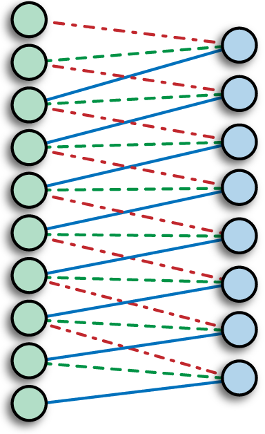
- Parameter sharing (same color = same weight)
- Far fewer weights to deal with versus dense layer.
Implements $\sigma(\mathbf W^T \mathbf x + \mathbf b)$ where $\mathbf W$ has a certain structure
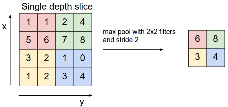
Pooling Layer
Convolutional neural networks (CNN) for Sequences
Dominant achitecture type for processing images
Not immediately obvious that would work well for text, but major advantages in efficiency and speed allow use of many layers and good performance when adapted for text processing
Kim 2014: treat text as a sequence of finite length
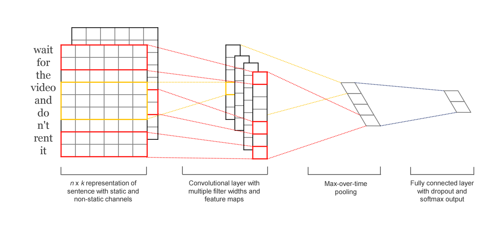
The next layer performs convolutions over the embedded word vectors using multiple filter sizes. For example, sliding over 3, 4 or 5 words at a time.
Next, the result of the convolutional layer is max-pooled into a long feature vector.
Create a classification prediction with a softmax layer.
import numpy as np
import tensorflow as tf
from tensorflow import keras
print("TF version: ", tf.__version__)
print("Keras version: ", keras.__version__)
from tensorflow.keras.datasets import imdb

max_features = 10000  # number of words to consider as features
max_len = 500  # cut texts after this number of words (among top max_features most common words)

print('Loading data...')
(x_train, y_train), (x_test, y_test) = imdb.load_data(num_words=max_features)
print(len(x_train), 'train sequences')
print(len(x_test), 'test sequences')
from tensorflow.keras.preprocessing import sequence

print('Pad sequences (samples x time)')
x_train = sequence.pad_sequences(x_train, maxlen=max_len)
x_test = sequence.pad_sequences(x_test, maxlen=max_len)

print('x_train shape:', x_train.shape)
print('x_test shape:', x_test.shape)
print('y_train shape:', y_train.shape)
print('y_test shape:', y_test.shape)
from tensorflow.keras.models import Sequential
from tensorflow.keras import layers

model = Sequential()
model.add(layers.Embedding(max_features, 128, input_length=max_len))
model.add(layers.Conv1D(32, 7, activation='relu'))
model.add(layers.MaxPooling1D(5))
model.add(layers.Conv1D(32, 7, activation='relu'))
model.add(layers.GlobalMaxPooling1D())
model.add(layers.Dense(1))

model.summary()
model.compile(loss='binary_crossentropy',
              metrics=['acc'])

history = model.fit(x_train, y_train,
                    epochs=10,
                    batch_size=128,
                    validation_split=0.2)
acc = history.history['acc']
val_acc = history.history['val_acc']
loss = history.history['loss']
val_loss = history.history['val_loss']

epochs = range(len(acc))

plt.plot(epochs, acc, 'bo', label='Training acc')
plt.plot(epochs, val_acc, 'b', label='Validation acc')
plt.title('Training and validation accuracy')
plt.legend()

plt.figure()

plt.plot(epochs, loss, 'bo', label='Training loss')
plt.plot(epochs, val_loss, 'b', label='Validation loss')
plt.title('Training and validation loss')
plt.legend();

