Unstructured Data & Natural Language Processing

Topic 8: Recurrent Neural Networks

This topic:

1. Background
2. Recurrent Networks
3. Architectures
4. Autoregressive text generation

Reading:

• J&M Ch 7 (Neural Networks and Neural Language Models)
• J&M Ch 9 (Sequence Processing with Recurrent Networks)
• J&M Ch 10 (Encoder-Decoder Models, Attention, and Contextual Embeddings)
• Young et al, "Recent trends in deep learning based natural language processing" 2018
• Sebastian Ruder, "A Review of the Neural History of Natural Language Processing" 2018

I. Background

Machine Learning Framework using Sklearn

1. Given training data $(\mathbf x_{(i)},y_i)$ for $i=1,...,m$ --> lists of samples $\verb|X|$ and labels $\verb|y|$

2. Choose a model $f(\cdot)$ where we want to make $f(\mathbf x_{(i)})\approx y_i$ (for all $i$) --> choose sklearn estimator to use

3. Define a loss function $L(f(\mathbf x), y)$ to minimize by changing $f(\cdot)$ ...by adjusting the weights --> default choices for estimators, sometimes multiple options

Deep Learning

Very flexible machine learning methods(s). I.e. there are many new options and variations to choose

1. Make up an architecture - choose layers and their parameters - define custom $f(\mathbf x_{(i)})$

2. Choose a Loss function - how compute error for $f(\mathbf x_{(i)}) \ne y_i$

3. Choose a optimization method - many variants of same basic method

4. Choose "regularization" tricks to prevent overfitting

5. Handle other important details like initializing and normalizing data

Multilayer (Artificial) Neural Networks - "Feed forward"

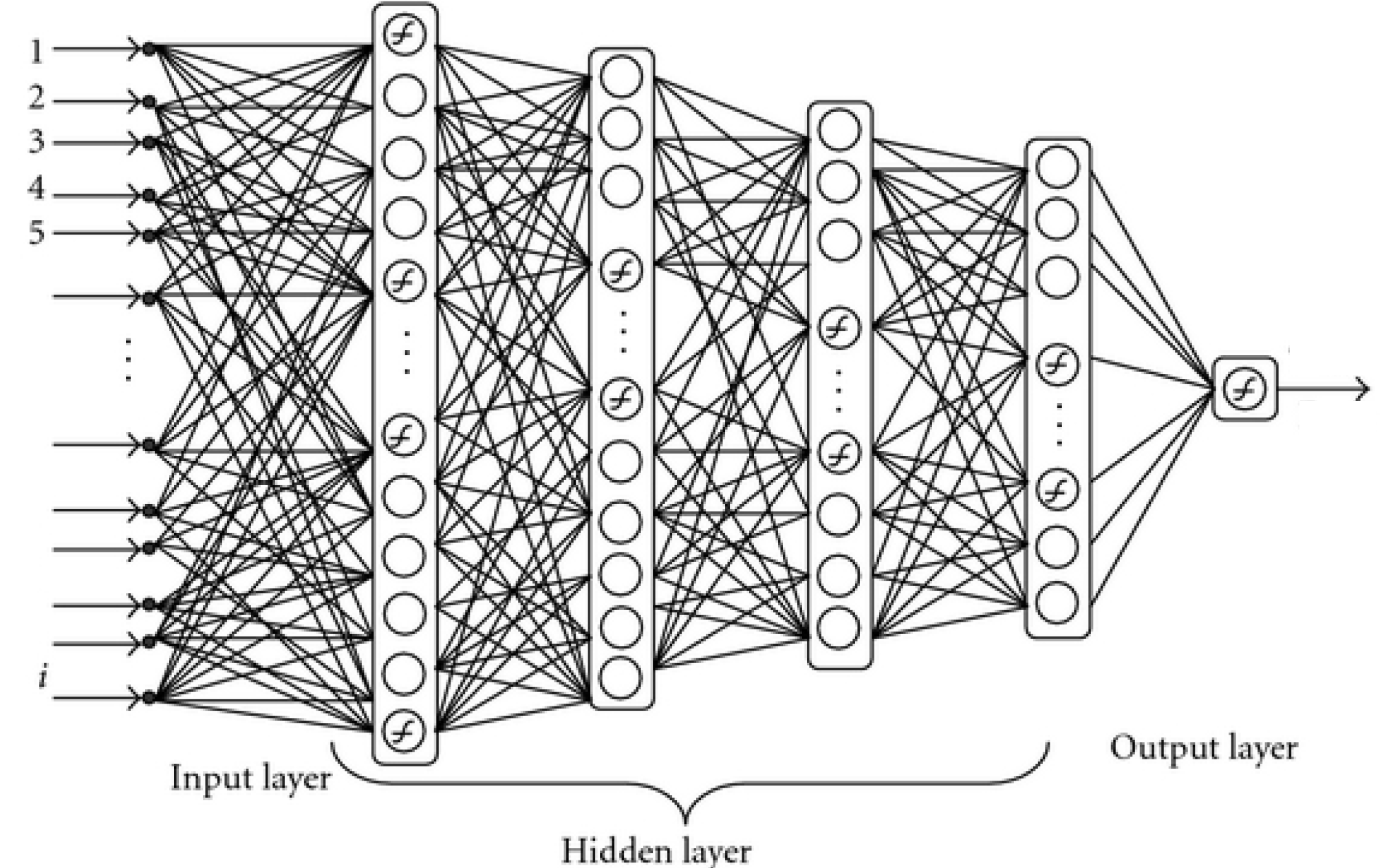
This is just a big complex model that computes $y = f(\mathbf x)$

Using a (fixed-length) sequence of words as inputs

Notice output shape was 3D, because each sample consisted of a list of words, each embedded to a vector

For each word in an input consisting of $$\mathbf h(\mathbf x) = \sigma(\mathbf z) = \sigma(\mathbf W^T \mathbf x + \mathbf b) = [\mathbf E^T \mathbf x^{(1)},\mathbf E^T \mathbf x^{(2)},...,\mathbf E^T \mathbf x^{(N)}]$$

"Flatten" layer converted this to a single concatenated vector

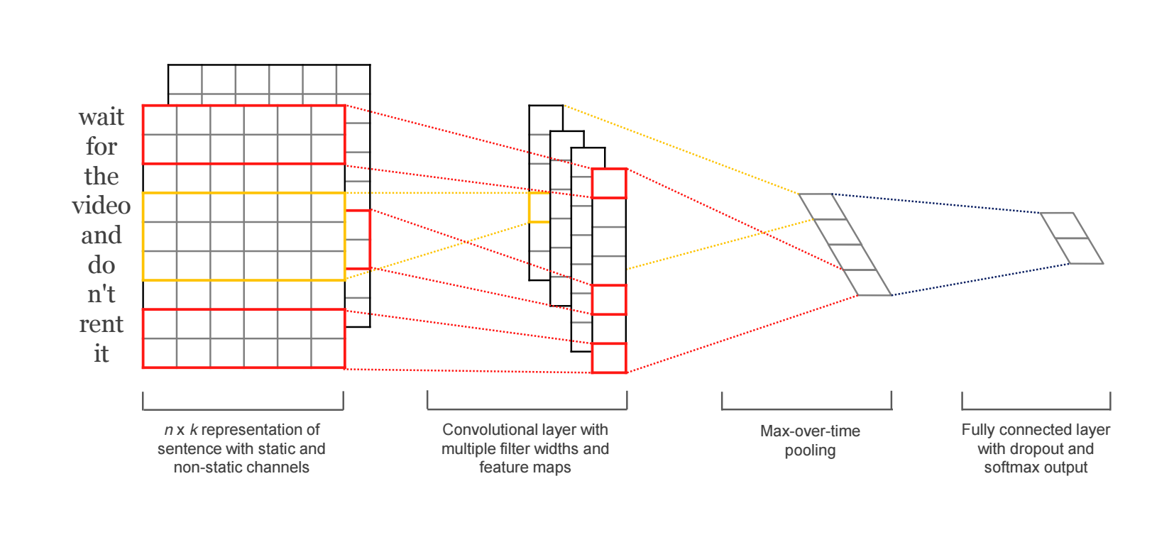
Convolutional neural networks (CNN) for Sequences

Dominant achitecture type for processing images

Not immediately obvious that would work well for text, but major advantages in efficiency and speed allow use of many layers and good performance when adapted for text processing

Kim 2014: treat text as a sequence of finite length

II. Recurrent Networks

Language is an inherently temporal phenomenon.

• continuous input streams of indefinite length
• machine learning approaches we’ve studied for sentiment analysis and other classification tasks do not have this temporal nature.

Feed-forward neural networks

• employ fixed-size input vectors with associated weights to capture all relevant aspects of an example at once.
• makes it difficult to deal with sequences of varying length, and they fail to capture important temporal aspects of language
• including when applied to neural language models - use a work-around by windowing neighboring inputs

Drawbacks of windowing approach

• limits the context from which information can be extracted, as with Markov approaches
• makes it difficult for networks to learn systematic patterns arising from phenomena like constituency (breaking sentences into phrases)

Recurrent neural network (RNN)

• Any network that contains a cycle within its network connections.
• Powerful, but difficult to reason about and train
• Certain constrained architectures are extremely effective when applied to spoken and written language
• Elman Networks(Elman, 1990) a.k.a. simple Elman Networks recurrent networks

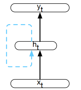
Simple recurrent neural network after Elman (Elman, 1990). The hidden layer includes a recurrent connection as part of its input. That is, the activation value of the hidden layer depends on the current input as well as the activation value of the hidden layer from the previous time step.

Simple recurrent neural network illustrated as a feedforward network.

\begin{align} \mathbf h_t &= g(\mathbf U \mathbf h_{t−1}+\mathbf W \mathbf x_t) \\ \mathbf y_t &= f(\mathbf V \mathbf h_t) = softmax(\mathbf V \mathbf h_t) \end{align}

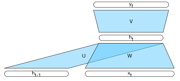
Loop unrolling

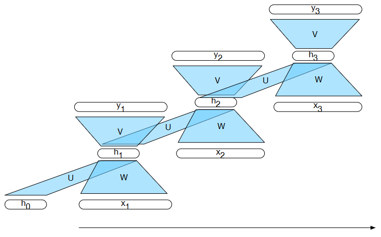
A simple recurrent neural network shown unrolled in time. Network layers are copied for each time step, while the weights $\mathbf U$, $\mathbf V$ and $\mathbf W$ are shared in common across all time steps

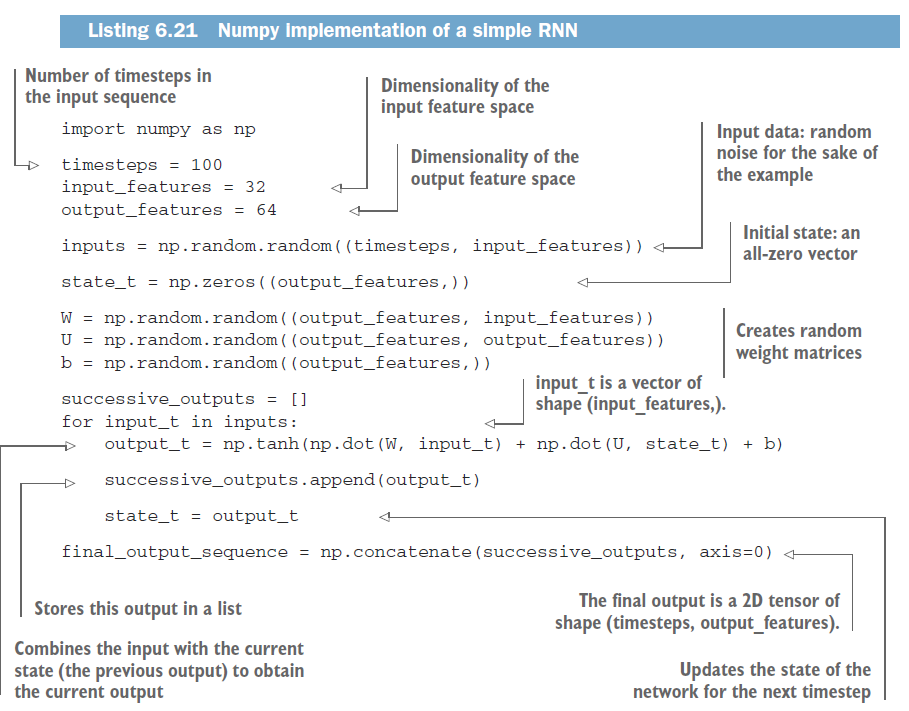
Keras Simple RNN

Applications of Recurrent Neural Networks

Effective approach to

• language modeling,
• sequence labeling tasks such as part-of-speech tagging
• sequence classification tasks such as sentiment analysis and topic classification.

Form the basis for sequence-to-sequence approaches (Ch. 10 and 11)

• summarization
• machine translation
• question answering.

Autoregressive text generation... demo later

Language Models

Goal: compute the conditional probability of the next word in a sequence given the preceding words $P(w_{n}|w_1^{n−1})$

$N$-gram models and feedforward networks with sliding windows both model this

The quality of a model is largely dependent on the size ofthe context and how effectively the model makes use of it.

Both make limited approximation $P(w_{n}|w_1^{n−1}) \approx P(w_n|w_{n-N+1}^{n−1})$

Recurrent models

• Do not make limited-sequence approximation.
• Current state depends on previous state.
• Previous state depending on state before that.
• Etc, all the way back to first input (initization states).
• I.e. Recurrent language models all preceding data to estimate $P(w_{n}|w_1^{n−1})$

Recurrent Neural Language models

\begin{align} P(w_{n}|w_1^{n−1}) &= y_n \\ &= softmax(\mathbf V \mathbf h_n) \end{align}

For probability of sequence, combine probabilities of words

\begin{align} P(w_{1}^{n}) &= \prod_{k=1}^n P(w_{k}|w_1^{k−1}) \\ &= \prod_{k=1}^n y_k \end{align}

Recall chain rule of probability

Cross-entropy Loss

for a single example gives the negative log probability assigned to the correct class, which is the result of applying a softmax to the final output layer.

\begin{align} L_{CE} &= -\log\hat{y}_i \\ &= -\log\frac{e^{z_i}}{\sum_{j=1}^K e^{z_j}} \end{align}

• the correct class $i$ is the word that comes next in the data
• $y_i$ is the probability assigned to that word
• the softmax is over the entire vocabulary,which has size $K$
• The weights in the network are adjusted to minimize the cross-entropy loss over the training set via gradient descent.

III. RNN Architectures

Stacked RNNs

• Stacking modules the same as with layers
• has been demonstrated in numerous tasks that stacked RNNs can outperform single-layer networks.
• as in deep feedforward networks, stacked RNNs can learn representations at differing levels of abstraction across layers

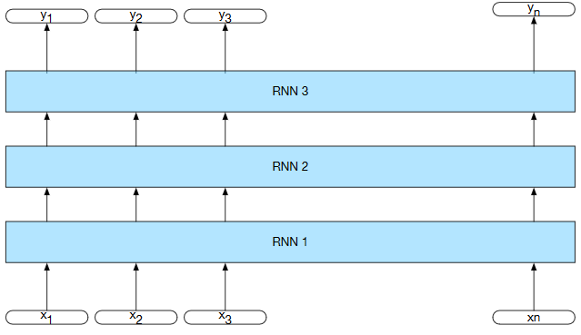
The output of a lower level serves as the input to higher levels with the output of the last network serving as the final output.

Forward & Backward RNNs

Simple recurrent network: the hidden state at time $t$ represents everything the network knows about the sequence up to that point in the sequence, i.e. using inputs preceding $t$

$$ h_t^{fwd}=RNN_{fwd}(x^t_1) $$

Can perform same training backward in time by reversing sequence and starting at end

$$ h_t^{bkwd}=RNN_{bkwd}(x^n_t) $$

Bidirectional RNN (Bi-RNN)

• Schuster and Paliwal, 1997
• proven to be effective for sequence classification.
• the final state naturally reflects more information about end of sentence than beginning
• Combining the forward and backward networks. E.g. by concatenating network outputs:

$$ h_t = h_t^{fwd} \oplus h_t^{bkwd} $$

• Can also use element-wise addition, multiplication, averaging

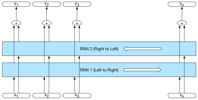
Bi-RNN. Separate models are trained in the forward and backward directions with the output of each model at each time point concatenated to represent the state of affairs at that point in time.

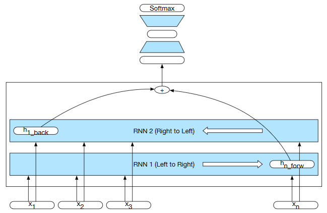
Bi-RNN for sequence classification. The final hidden units from the forward and backward passes are combined to represent the entire sequence. This combined representation serves as input to the subsequent classifier.

Difficulties in Simple RNN Architectures

• Hard to train RNNs for tasks that require a network to make use of information distant from the current point of processing.
• Weights that determine the values in the hidden layer must perform two tasks simultaneously:
  1. Provide information useful for the current decision
  2. Update and carry forward information required for future decisions
• Vanishing gradient problem - repeated multiplications during training, as determined by the length of the sequence. the gradients are eventually driven to zero

Example

The flights the airline was cancelling were full.

"was" should have probability of following "flight"

"were" also follows "flight" in sense, delayed due to phrase in middle

Learning approach

• Divide the context management problem into two subproblems:
  1. removing information no longer needed from the context - "forget"
  2. adding information likely to be needed for later decision making - "carry"

Manage this context rather than hard-coding a strategy into the architecture - "gates"

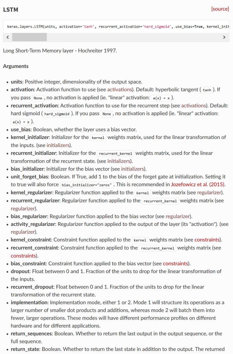
Long short-term memory (LSTM) networks

• Hochreiter and Schmidhuber 1997
• add an explicit context layer to the architecture (in addition to the usual recurrent hidden layer)
• use specialized neural units that make use of gates to control the flow of information into and out of the units that comprise the network layers.
• gates are implemented through the use of additional weights that operate sequentially on the input, and previous hidden layer, and previous context layers

Recall simple RNN layer

$$ h_t=\tanh(\mathbf U \mathbf h_{t−1}+ \mathbf W \mathbf x_t)$$

Starting point for LSTM...

$$ g_t=\tanh(\mathbf U_gh_{t−1}+ \mathbf W_g \mathbf x_t)$$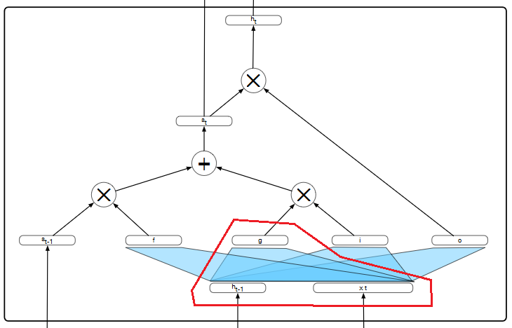

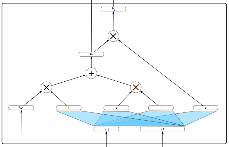
LSTM gates

Common design pattern for each gate

1. a feed-forward layer
2. a sigmoid activation function: 1 = open gate, 0 = closed gate
3. a pointwise multiplication with the layer being gated.

Forget gate

• Purpose: delete information from the context that is no longer needed.
• Computes a weighted sum of the previous state’s hidden layer and the current input
• passes that through a sigmoid to determine open/closed gate.
• This mask is then multiplied by the context vector to remove the information from context that is no longer required.

\begin{align} f_t &= σ(\mathbf U_f \mathbf h_{t−1}+ \mathbf W_f \mathbf x_t) \\ k_t & = c_{t−1}f_t \end{align}

Add gate

To select the information to add to the current context

\begin{align} i_t &= σ(\mathbf U_i \mathbf h_{t-1} + \mathbf W_i \mathbf x_t) \\ j_t & = g_{t} \odot i_t \end{align}

Update context

$$ c_t=j_t+k_t$$

Output gate

To decide what information is required for the current hidden state (as opposed to what information needs to be preserved for future decisions)

\begin{align} o_t &= σ(\mathbf U_0 \mathbf h_{t-1} + \mathbf W_0 \mathbf x_t) \\ h_t & = o_{t} \odot \tanh c_t \end{align}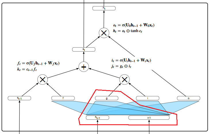

LSTM Drawbacks

• LSTMs introduce a considerable number of additional parameters to our recurrent networks.
• have 8 sets of weights to learn (i.e., the $\mathbf U$ and $\mathbf W$ for each of the 4 gates within each unit)
• whereas simple recurrent units only had 2.
• Training these additional parameters imposes a much significantly higher training cost.

Gated Recurrent Units (GRUs)

• Cho et al 2014
• Do not use a separate context vector,
• Reduce number of gates to 2
  1. reset gate $r$
  2. update gate $z$

\begin{align} r_t & = σ(\mathbf U_r \mathbf h_{t-1} + \mathbf W_r \mathbf x_t) \\ z_t & = σ(\mathbf U_z \mathbf h_{t-1} + \mathbf W_z \mathbf x_t) \end{align}

Reset used in gating recurrent input for intermediate output

$$ \hat{h}_t=\tanh\big(\mathbf U_t (\mathbf r_t\odot \mathbf h_{t−1}) + \mathbf W \mathbf x_t\big)$$

Update gate used in combining with recurrent output $$ h_t= (1−z_t)h_{t−1}+z_t ̃\hat{h}_t $$

Neural Unit Recap

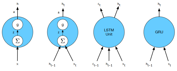
Feed-forward, Simple RNN, LSTM, GRU

Complexity increase encapsulated within unit

Outward complexity boils down to recurrent connection(s), unroll loop for optimization

IV. Autoregressive Text Generation

Autoregressive Text Generation

Shannon’s method (Shannon, 1951) used to use to generate random sentences in Ch. 3

1. sample first word in the output from the softmax distribution that results from using the beginning of sentence marker < s > as the first input.
2. Use the word embedding for that first word as the input to the network at the next time step, and then sample the next word in the same fashion.
3. Continue generating until the end of sentence marker </ s > is sampled or a fixed length limit is reached.

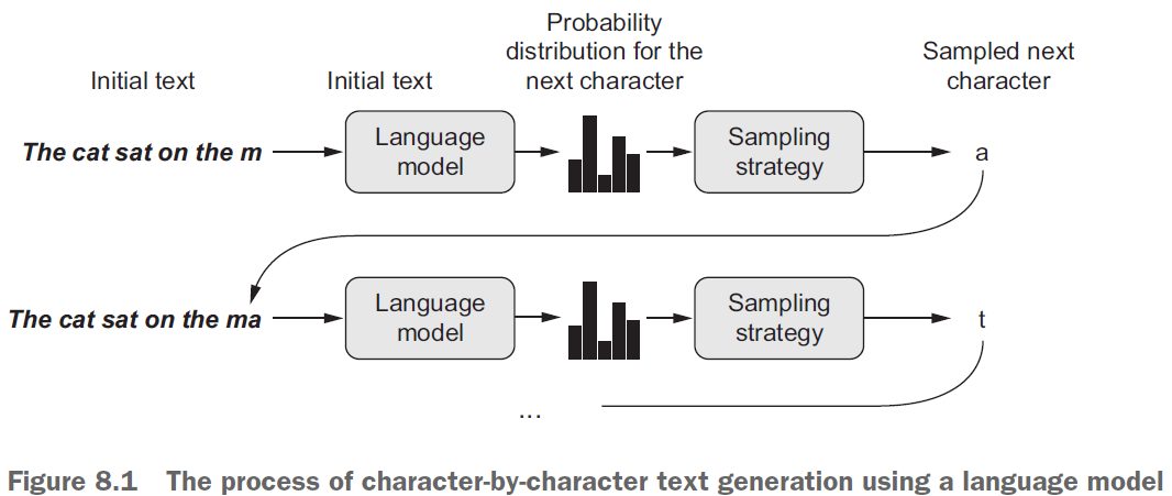
Text generation

Use characters as your tokens

Use the predicted character as part of the next input sequence to predict subsequent character

keep repeating this process

RNN Text generation - history & prefix

1. Apply RNN to generate dist over possible next words (softmax values)
2. Choose word from dist (e.g. max likelihood)
3. Feed word back in as next input (autoregressive) -- but use certain length "prefix" first

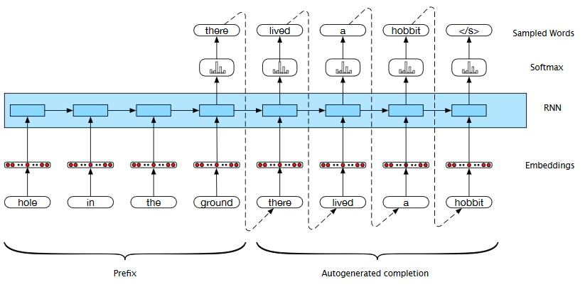
Recall must embed word when chosen for feedback

import numpy as np

path = keras.utils.get_file('nietzsche.txt',origin='https://s3.amazonaws.com/text-datasets/nietzsche.txt')
text = open(path).read().lower()
print('Corpus length:', len(text))

Downloading data from https://s3.amazonaws.com/text-datasets/nietzsche.txt
606208/600901 [==============================] - 1s 2us/step
Corpus length: 600893

# Length of extracted character sequences
maxlen = 60

# We sample a new sequence every `step` characters
step = 3

# This holds our extracted sequences
sentences = []

# This holds the targets (the follow-up characters)
next_chars = []

for i in range(0, len(text) - maxlen, step):
    sentences.append(text[i: i + maxlen])
    next_chars.append(text[i + maxlen])
print('Number of sequences:', len(sentences))

# List of unique characters in the corpus
chars = sorted(list(set(text)))
print('Unique characters:', len(chars))
# Dictionary mapping unique characters to their index in `chars`
char_indices = dict((char, chars.index(char)) for char in chars)

# Next, one-hot encode the characters into binary arrays.
print('Vectorization...')
x = np.zeros((len(sentences), maxlen, len(chars)), dtype=np.bool)
y = np.zeros((len(sentences), len(chars)), dtype=np.bool)
for i, sentence in enumerate(sentences):
    for t, char in enumerate(sentence):
        x[i, t, char_indices[char]] = 1
    y[i, char_indices[next_chars[i]]] = 1

Number of sequences: 200278
Unique characters: 57
Vectorization...