Unstructured Data & Natural Language Processing
Topic 9: Sequence Labeling
Sequence Labeling
Category of Methods
Goal: to assign a label chosen from a small fixed set of labels to each element of a sequence
Canonical Example: Part-of-speech (POS) tagging
Conditional random fields (CRF; Lafferty et al., 2001)
- one of the most influential classes of sequence labelling methods
- won the Test-of-time award at ICML 2011.
- A CRF layer is a core part of current state-of-the-art models for sequence labelling problems with label interdependencies such as named entity recognition (Lample et al., 2016)
Structure prediction.
- Goal: take an input sequence and produce some kind of structured output, such as a parse tree or meaning representation.
- One possible approach: learn a sequence of actions, or operators, which when executed would produce the desired structure.
- Instead of predicting a label for each element of an input sequence, the network is trained to select a sequence of actions, which when executed in sequence produce the desired output.
- Example: transition-based parsing which borrows the shift-reduce paradigm from compiler construction. (Ch. 15 dependency parsing)
I. Part-of-Speech Tagging
Dionysius Thrax of Alexandria (c.100 B.C.)
eight parts of speech:
- noun - most people, places, things, verb-like terms ("eating dinner is good")
- verb - actions and processes
- pronoun - she, who, I, others
- preposition - occur before noun phrases, {on, under, to, with, by, at, ...}
- adverb - modify verbs and adjectives
- conjunction - and, but, or, as, if, when
- participle
- article
The basis for practically all subsequent part-of-speech descriptions of most European languages, suggesting deep importance
Modern tagsets may use many more tags. Penn treebank = 45
Part-of-Speech Tagging
the process of assigning a part-of-speech marker to each word in an input text
Also known as...
- POS
- Word classes
- syntactic categories
Value of POS tags
- Knowing whether a word is a noun or averb tells us about likely neighboring words (nouns are preceded by determiners and adjectives, verbs by nouns) and syntactic structure (nouns are generally part of noun phrases),
- making part-of-speech tagging a key aspect of parsing (Chapter 12)
- Parts of speech are useful features for labeling named entities like people or organizations in information extraction (Chapter 17), or for coreference resolution (Chapter 21).
- can even play a role in speech recognition or synthesis, e.g., the word "content" is pronounced CONtent when it is a noun and conTENT when it is an adjective
Approaches to POS tagging
- generative — Hidden Markov Model (HMM)
- discriminative — the Maximum Entropy Markov Model (MEMM).
- Recurrent NN's (chapter 9 in J&M)
All three methods have roughly equal performance but different tradeoffs
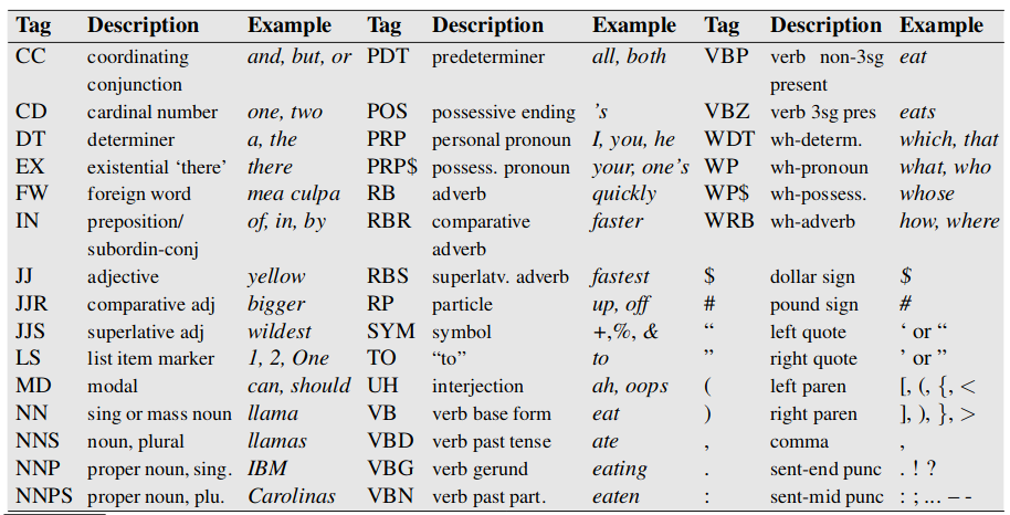
Penn Treebank tagset
- Marcus et al,1993
- used to label many corpora
- parts of speech are generally represented by placing the tag after eachword, delimited by a slash
Examples
(8.1) The/DT grand/JJ jury/NN commented/VBD on/IN a/DT number/NN of/IN other/JJ topics/NNS ./.
(8.2)There/EX are/VBP 70/CD children/NNS there/RB
(8.3) Preliminary/JJ findings/NNS were/VBD reported/VBN in/IN today/NN ’s/POS New/NNP England/NNP Journal/NNP of/IN Medicine/NNP ./.
Three main tagged corpora used for training and testing part-of-speech taggers for English
Brown corpus - a million words of samples from 500 written texts from different genres published in the United States in 1961
WSJ corpus contains a million words published in the Wall Street Journal in 1989.
Switchboard corpus consists of 2 million words of telephone conversations collected in 1990-1991.
Penn Treebank
45 tags were collapsed from 87-tag Brown tagset
designed for a treebank in which sentences were parsed (making trees), and so it leaves off syntactic information recoverable from the parse tree
Universal POS tag set of the Universal Dependencies project
- Nivre et al, 2016
- used when building systems that can tag many languages
Difficulties & Nuances in POS Tagging
Please read J&M Chapter 8 section 1.
Some examples in the following slides...
Adjective Language variations
Interchange with Verbs: "beautiful" becomes "to be beautiful"
Interchange with nouns: "I like rice" vs "rice is likeable"
Words of Unique (more or less) Function
- interjections (oh, hey, alas, uh, um),
- negatives (no, not),
- politeness markers (please, thank you),
- greetings (hello, goodbye),
- the existential there (there are two on the table)
- others.
These classes may be distinguished or lumped together as interjections or adverbs depending on the purpose of the labeling.
Closed and open class words
Closed = fixed (relatively) vocabulary, versus Open = able to add new words
Closed classes generally function words (of, it, and, you), important to structure. New prepositions are rarely coined.
Nouns and verbs are open classes. new nouns and verbs like iPhone or fax are continually being created or borrowed. Also adjectives and adverbs.
Any given speaker or corpus may have different open class words, but all speakers of a language, and sufficiently large corpora, likely share the set of closed class word
Proper versus Common nouns
Proper nouns
- Regina, Colorado, IBM,
- are names of specific persons or entities.
- In English, they generally aren’t preceded by articles (e.g., the book is upstairs, vs Regina is upstairs).
- In written English, proper nouns are usually capitalized.
Common nouns
- Divided (in many languages, including English), into count nouns and mass nouns.
- Count nouns - both the singular and plural (goat/goats, relationship/relationships) and they can be counted (one goat, two goats).
- Mass nouns - homogeneous group (snow, salt, and communism)
- Mass nouns can also appear without articles where singular count nouns cannot ("Snow is white" but not "Goat is white").
Adverbs - Heterogenous category
"a hodge-podge in both form and meaning"
Directional adverbs or locative adverbs (home, here, downhill)
Degree adverbs (extremely,very,somewhat)
Manner adverbs (slowly,slinkily,delicately)
Temporal adverbs (yesterday,Monday).
some adverbs (e.g., temporal adverbs like Monday) are tagged in some "tagging schemes as nouns.
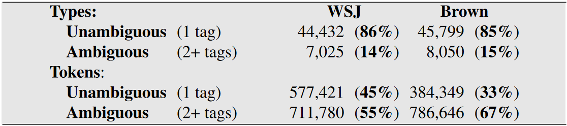
Disambiguation
Disambiguation task - resolving ambiguous words (book a flight vs. read a book).
- ambiguous words are only 14-15% of the vocabulary
- but are very common words 55-67% of word tokens in running text
Baseline algorithm for part-of-speech tagging
given an ambiguous word, choose the tag which is most frequent in the training corpus.
Accuracy training on WSJ corpus and test on sections 22-24 of the same corpus:
- most-frequent-tag baseline achieves an accuracy of 92.34%.
- the state of the art on this dataset is around 97% tag accuracy,
- achievable by most algorithms (HMMs, MEMMs, neural networks, rule-based).
Consider how this baseline algorithm relates to describing text with $N$-grams.
Part-of-speech (POS) tagging via RNN
inputs are word embeddings and the outputs are tag probabilities generated by a softmax layer over the tagset
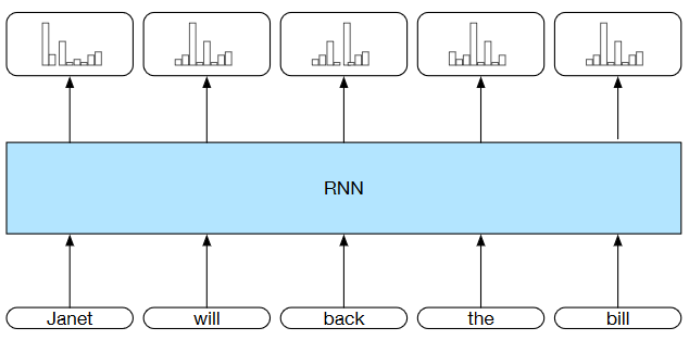
- Part-of-speech tagging as sequence labeling with a simple RNN.
- Pre-trained word embeddings serve as inputs
- a softmax layer provides a probability distribution over the part-of-speech tags as output at each time step.
II. NER
Named Entity Recognition (NER)
- Application of sequence labeling to span-recognition problem
- the problem of finding all the spans in a text that correspond to names of people, places or organizations
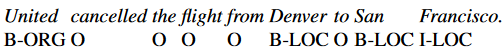
IOB encoding
- Ramshaw and Marcus, 1995
- $B$ - Begin - label for any token that begins a span of interest
- $I$ - Inside - label for tokens that occur inside a span
- $O$ - Outside - label for tokens outside of any span of interest
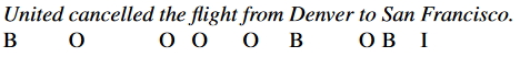
- Here the spans of interest are United, Denver and San Francisco
- Can specialize the $B$ and $I$ tags to represent each of the more specific classes (e.g. organization, location, ...)
- expanding the tagset from 3 tags to $2N+1$, where $N$ is the number of classes we’re interested in.
III. Sequence Classification with RNNs
Sequence Classification
Entire sequences of text are classified as belonging to one of a small number of categories.
- sentiment analysis
- document-level topic classification
- spam detection
- message routing for customer service applications
- deception detection
Simple RNN Approach
- Text to be classified is passed through the RNN a word at a time generating a new hidden layer at each time step.
- The hidden layer output the final element of the text $\mathbf h_n$ as a compressed representation of the entire sequence.
- $\mathbf h_n$ input to subsequent feedforward network that chooses a class via a softmax over the possible classes
- the loss function used to train the weights in the network is based entirely on the final text classification task - end-to-end training
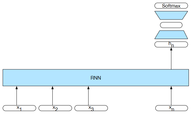
Sequence classification using a simple RNN combined with a feedforward network. The final hidden state from the RNN is used as the input to a feedforward network thatperforms the classification.
LSTM for IMDB
from keras.datasets import imdb
from keras.preprocessing import sequence

max_features = 10000  # number of words to consider as features
maxlen = 500  # cut texts after this number of words (among top max_features most common words)
batch_size = 32

print('Loading data...')
(input_train, y_train), (input_test, y_test) = imdb.load_data(num_words=max_features)
print(len(input_train), 'train sequences')
print(len(input_test), 'test sequences')

print('Pad sequences (samples x time)')
input_train = sequence.pad_sequences(input_train, maxlen=maxlen)
input_test = sequence.pad_sequences(input_test, maxlen=maxlen)
print('input_train shape:', input_train.shape)
print('input_test shape:', input_test.shape)
from keras.models import Sequential
from keras.layers import LSTM
from keras.layers import Dense
from keras.layers import Embedding

model = Sequential()
model.add(Embedding(max_features, 32))
model.add(LSTM(32))
model.add(Dense(1, activation='sigmoid'))

model.compile(optimizer='rmsprop',
              loss='binary_crossentropy',
              metrics=['acc'])
history = model.fit(input_train, y_train,
                    epochs=10,
                    batch_size=128,
                    validation_split=0.2)