Deep Learning

Keith Dillon
Fall 2019

Topic 3: Universal Approximation

This topic:

1. Artificial Neurons
2. Network Diagrams
3. Learning boolean functions
4. Universal function approximation

Reading:

• Alpaydin Chapter 11 (Multilayer perceptron)
• Geron Chapter 10 (Artificial Neural Networks)
• Geron Appendix (Artificial Neural Networks)

Outcomes

• Develop skill in working with network diagrams - relate math to diagram
• Build intuition for how we might use perceptrons and networks to perform tasks

I. Artificial Neural Networks

Marr Levels of Analysis

Marr (1982), understanding an information processing system has three levels, called the levels of analysis:

1. Computational theory corresponds to the goal of computation and an abstract definition of the task.
2. Representation and algorithm is about how the input and the output are represented and about the specification of the algorithm for the transformation from the input to the output.
3. Hardware implementation is the actual physical realization of the system.

Example: sorting

1. The computational theory is to order a given set of elements.
2. The representation may use integers
3. the algorithm may be Quicksort.

A.I. by imitating the brain

"The brain is one hardware implementation for learning or pattern recognition."

1. If from this particular implementation, we can do reverse engineering and extract the representation and the algorithm used
2. if from that in turn, we can get the computational theory,
3. we can then use another representation and algorithm, and in turn a hardware implementation more suited to the means and constraints we have.

Neural Networks as a Paradigm for Parallel Processing

There are mainly two paradigms for parallel processing:

1. Single instruction, multiple data (SIMD) - all processors execute the same instruction but on different pieces of data
2. Multiple instruction, multiple data (MIMD) machines - different processors may execute different instructions on different data

"Neural instruction, multiple data" (NIMD) machines

• processors are a little bit more complex than SIMD processors but not as complex as MIMD processors
• simple processors with a small amount of local memory where some parameters can be stored
• Each processor implements a fixed function and executes the same instructions as SIMD processors; but by loading different values into the local memory, they can be doing different things and the whole operation can be distributed over such processors
• Each processor corresponds to a neuron, local parameters correspond to its synaptic weights, and the whole structure is a neural network

"The problem now is to distribute a task over a network of such processors and to determine the local parameter values"

"Learning: We do not need to program such machines and determine the parameter values ourselves if such machines can learn from examples."

"Thus, artificial neural networks are a way to make use of the parallel hardware we can build with current technology and—thanks to learning— they need not be programmed. Therefore, we also save ourselves the effort of programming them."

"Keep in mind that the operation of an artificial neural network is a mathematical function that can be implemented on a serial computer"

Artificial Neural Networks and Deep Learning

ANNs are the method used in Deep Learning.

They are versatile, powerful, and scalable,

Ideal to tackle large and highly complex Machine Learning tasks, such as

• classifying billions of images (e.g., Google Images),
• powering speech recognition services (e.g., Apple’s Siri),
• recommending the best videos to watch to hundreds of millions of users every day (e.g., YouTube),
• learning to beat the world champion at the game of Go by examining millions of past games and then playing against itself (DeepMind’s AlphaGo).

History, part 1

• first introduced in 1943 by the neurophysiologist Warren McCulloch and the mathematician Walter Pitts.
• landmark paper, “A Logical Calculus of Ideas Immanent in Nervous Activity,”
• presented a simplified computational model of how biological neurons might work together in animal brains to perform complex computations using propositional logic.
• This was the first artificial neural network architecture.

McCulloch and Pitts simple model of the biological neuron

• performed logical computations
• later became known as an artificial neuron
• has one or more binary (on/off) inputs
• one binary output.
• simply activates its output when more than a certain number of its inputs are active
• even with such a simplified model it is possible to build a network of artificial neurons that computes any logical proposition you want

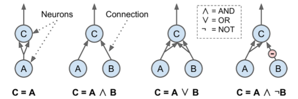
The multi-arrow inputs imply a double weight input sufficient to activate post-synaptic neuron alone.

History, part 2

• Early successes of ANNs until the 1960s led to the widespread belief that we would soon be conversing with truly intelligent machines.
• Rosenblatt (1962) proposed the perceptron model and a learning algorithm in 1962.
• Minsky and Papert (1969) showed the limitation of single-layer perceptrons, for example, the XOR problem, and since there was no algorithm to train a multilayer perceptron with a hidden layer at that time, the work on artificial neural networks almost stopped except at a few places.
• Promise unfulfilled, first dark age of ANN's

The Perceptron

• Invented by Frank Rosenblatt in 1957.
• a slightly different artificial neuron called a linear threshold unit (LTU)
• the inputs and output are now numbers (instead of binary on/off values)
• each input connection is associated with a weight.

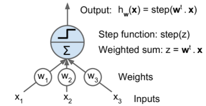
Operation

1. computes a weighted sum of its inputs $z = w_1 x_1 + w_2 x_2 + ... + w_n x_n = \mathbf w^T \mathbf x$,
2. then applies a step function to that sum and outputs the result: $h_{\mathbf w}(\mathbf x) = \text{step}(\mathbf z) = \text{step}(\mathbf w^T \mathbf x)$

Step functions

Most common step function used in Perceptrons is the Heaviside step function

$$ \text{heaviside}(z) = \begin{cases} 0, &\text{if $z<0$} \\ 1, &\text{if $z \ge 0$} \end{cases} $$

Sometimes the sign function is used instead.

$$ \text{sgn}(z) = \begin{cases} -1, &\text{if $z<0$} \\ 0, &\text{if $z=0$} \\ 1, &\text{if $z > 0$} \end{cases} $$

History, part 3

• Early 1980s there was a revival of interest in ANNs as new network architectures were invented and better training techniques were developed
• The renaissance of neural networks came with the paper by Hopfield (1982). This was followed by the two-volume parallel distributed processing (PDP) book written by the PDP Research Group (Rumelhart, McClelland, and the PDP Research Group 1986).
• 1990s, powerful alternative Machine Learning techniques like SVM's took over spotlight due to superior results and theory

1990s+

Currently new wave of interest, good reasons to believe that this one is different and will have a much more profound impact on our lives:

• There is now a huge quantity of data available to train neural networks, and ANNs frequently outperform other ML techniques on very large and complex problems.
• The tremendous increase in computing power since the 1990s now makes it possible to train large neural networks in a reasonable amount of time. This is in part due to Moore’s Law, but also thanks to the gaming industry, which has produced powerful GPU cards by the millions.
• The training algorithms have been improved. To be fair they are only slightly different from the ones used in the 1990s, but these relatively small tweaks have a huge positive impact.
• Some theoretical limitations of ANNs have turned out to be benign in practice. For example, many people thought that ANN training algorithms were doomed because they were likely to get stuck in local optima, but it turns out that this is rather rare in practice (or when it is the case, they are usually fairly close to the global optimum).
• ANNs seem to have entered a virtuous circle of funding and progress. Amazing products based on ANNs regularly make the headline news, which pulls more and more attention and funding toward them, resulting in more and more progress, and even more amazing products

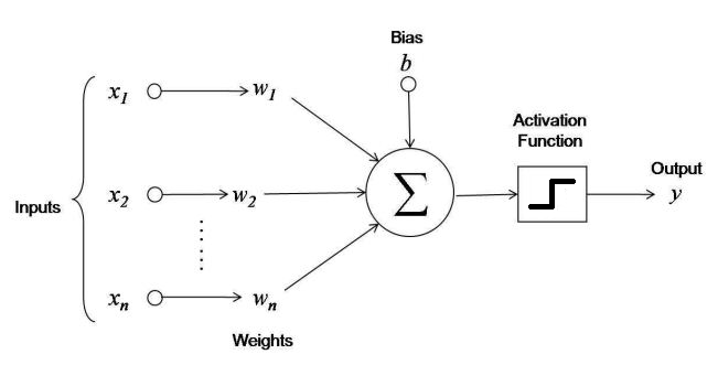
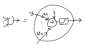
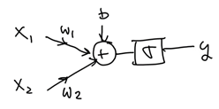
The artificial neuron - Perceptron

The basic processing element

1. inputs
2. Bias
3. weights
4. Activation function

II. Network Diagrams

Diagram levels of detail

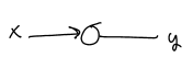
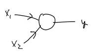
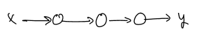
1. Explicit signal processing diagrams
2. Complex nodes
3. Functional blocks

All represent mathematical functions and their composition

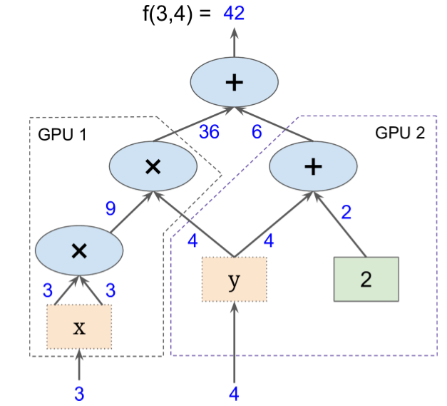
Computation Graph

Break computation into a tree of elementary operations ("ops") and the flow of variables from input to outputs

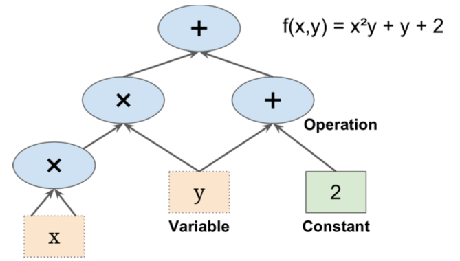
• Operations can take any number of inputs and produce any number of outputs
• "+" operation takes two inputs and produces one output

Write the composite functions for these subgraphs

write the mathematical equation for the following diagram

Given:

write the mathematical equation for the following diagram

Given:

write the mathematical equation for the following diagram

Given:

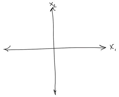
Hyperplane classification

Write the mathematical function implemented by a perceptron

Picture decision surface for following 2-input cases...

Write the equation and Draw the output regions for this network (given parameters):

What about this one?

And what about your IRIS classifier?

Moar...

III. Programming Boolean Functions

Boolean Functions

• inputs are binary
• output is 1 if the corresponding function value is true,
• output is 0 otherwise

AND

Logical AND can be implemented with a perceptron

$$ y = \sigma(x_1 + x_2 − 1.5) $$

OR

Logical OR can also be implemented with a perceptron

$$ y = \sigma(x_1 + x_2 − 0.5) $$

XOR

Logical XOR cannot be implemented with a perceptron

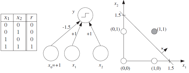
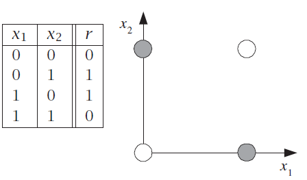
Linear separability

A perceptron uses a linear decision boundary (a.k.a. decision surface)

An XOR requires a nonlinear decision boundary

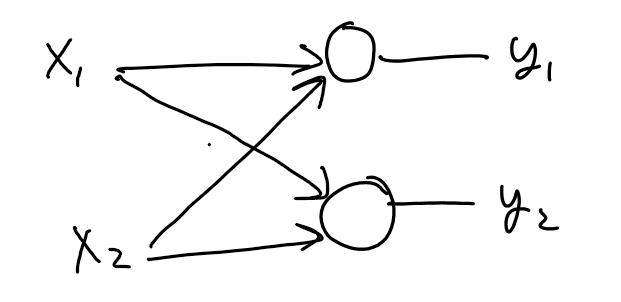
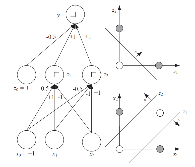
XOR Solution: Use Multiple Layers

IV. The Universal Approximator

Boolean case

"We can represent any Boolean function as a disjunction of conjunctions, and such a Boolean expression can be implemented by a multilayer perceptron with one hidden layer."

$x_1$ XOR $x_2$ = ($x_1$ AND ∼$x_2$) OR (∼$x_1$ AND $x_2$)

• Disjunction - OR
• Conjunction - AND
• Disjunction of Conjunctions - First AND of inputs, followed by OR of the results

I.e. form function as composition of elementary functions then implement elementary functions with perceptrons

Composition of perceptrons = MLP

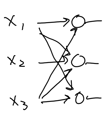
Proof of existence of solution for any boolean function

"for every input combination where the output is 1, we define a hidden unit that checks for that particular conjunction of the input. The output layer then implements the disjunction."

In other words, we can implement any truth table by making a perceptron that implements each row.

Generally an impractical approach (up to $2d$ hidden units may be necessary when there are $d$ inputs),

Proves universal abiility of MLP to describe any boolean function with a single hidden layer

Practice Example

A random truth table.

Suppose $x_1$, $x_2$, and $x_3$ are features of an email (e.g. contains a certain word or not)

$y$ is the prediction that the email is spam or not based on the features

$x_1$	$x_2$	$x_3$	$y$
0	0	0	1
0	0	1	0
0	1	0	0
0	1	1	1
1	0	0	1
1	0	1	0
1	1	0	1
1	1	1	1

Continuous case

Proof of universal approximation with two hidden layers:

1. For every input case or region, that region can be delimited by hyperplanes on all sides using hidden units on the first hidden layer
2. A hidden unit in the second layer then ANDs them together to bound the region
3. We then set the weight of the connection from that hidden unit to the output unit equal to the desired function value

Piecewise constant approximation of the function

Try implementing this one with a netral network

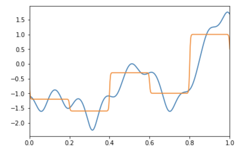
Single-hidden layer

It has been proven that an MLP with one hidden layer (with an arbitrary number of hidden units) can learn any nonlinear function of the input (Hornik, Stinchcombe, and White 1989).

I.e. even a Single Hidden Layer can achieve arbitrary decision boundaries

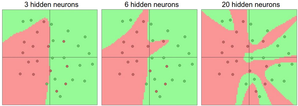
However the future of Neural Networks turned out to be "deep" stacks of layers...