Deep Learning

Keith Dillon
Fall 2019

Topic 4: Perceptron Training ("Learning")

This topic:

1. The Perceptron
2. Perceptron Learning Algorithm
3. Accuracy of Classification
4. Multi-category classification with multiple neurons

Reading:

• Chollet: Chapter 2
• GBC: Chapter 6

Outcomes

• An introduction to machine learning with neural networks using the simpest network and algorithm

• Develop skills in programming artificial neural networks and machine learning with them

Recap

• Thus far we have considered making perceptron and neural network classifiers by hand
• We also heard that it should be possible to make a network that can do anything "do-able", i.e. fit an arbitrary function with arbitrary accuracy, assuming the function exists, and we can make a network that has as many nodes as needed
• Now we consider the Machine Learning perspective, where we don't even know the function, we just have data which provides examples of inputs and outputs from the function
• We start with the perceptron again...

Outcomes

• A simple introduction to machine learning with neural networks (using the simpest network and algorithm)
• Develop skills in programming artificial neural networks and machine learning with them

1. Perceptron Function

1. input of some size
2. weights
3. Activation function

Create this in Python

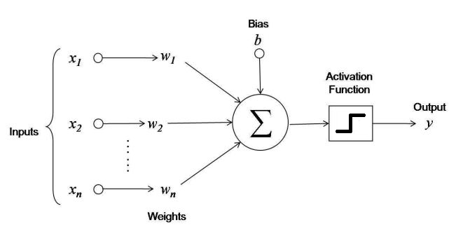
Operation

1. computes a weighted sum of its inputs $z = w_1 x_1 + w_2 x_2 + ... + w_n x_n + b= \mathbf w^T \mathbf x +b$,
2. then applies a step function to that sum and outputs the result: $h_{\mathbf w}(\mathbf x) = \text{step}(z) = \text{step}(\mathbf w^T \mathbf x +b)$

Activation function: Step functions

Most common step function used in Perceptrons is the Heaviside step function

$$ \text{heaviside}(z) = \begin{cases} 0, &\text{if $z<0$} \\ 1, &\text{if $z \ge 0$} \end{cases} $$

Sometimes the sign function is used instead.

$$ \text{sgn}(z) = \begin{cases} -1, &\text{if $z<0$} \\ 0, &\text{if $z=0$} \\ 1, &\text{if $z > 0$} \end{cases} $$

f([1,1],[2,2],3)

1

x = [1,2,3,4,5]
w = [6,7,8,9,0]

f(x,w,-10)

1

Machine Learning in a Nutshell

Machine Learning basically means methods that learn from data.

The most important class of methods are Supervised Learning

Here we will focus on using supervised learning for Classification

Given a training set consisting of :

• input samples $\mathbf x_i$ such as images, text strings, measurements of some features
• output labels $y_i$ corresponding to each input sample, such as cat vs. dog, disease vs. healthy, this is the sample's class
• Learn a function $f(\mathbf x) = y$ that can predict the label for a new unlabeled sample, i.e. classify it.

Classification discussion

Given a training set consisting of :

• input samples $\mathbf x_i$ such as images, text strings, measurements of some features
• output labels $y_i$ corresponding to each input sample, such as cat vs. dog, disease vs. healthy, this is the sample's class
• Learn a function $f(\mathbf x) = y$ that can predict the label for a new unlabeled sample, i.e. classify it.

Consider how this may be applied (what is $\mathbf x$, $y$, $f$, and what is "learned"?) in fields like:

• computer security
• online sales (i.e. amazon)
• finance

Perceptron as a Classifier

• A single perceptron can be used for simple linear binary classification.
• It computes a linear combination of the inputs and if the result exceeds a threshold, it outputs the positive class or else outputs the negative class (just like a Logistic Regression classifier or a linear SVM).
• For example, you could use a single perceptron to classify iris flowers based on the petal length and width
• also adding an extra bias feature $x_0 = 1$, instead of using a bias $b$
• Training an perceptron means finding the right values for $b$, $w_1$, $w_2$, ...

Hebbian Learning

• The Organization of Behavior, published in 1949 by Donald Hebb
• suggested that when a biological neuron often triggers another neuron, the connection between these two neurons grows stronger
• summarized by Siegrid Löwel in this catchy phrase: “Cells that fire together, wire together.”
• This rule became known as Hebb’s rule (or Hebbian learning); that is, the connection weight between two neurons is increased whenever they have the same output.

Perceptron Training

• Perceptrons are trained using a variant of Hebb's rule that takes into account the error made by the network
• it does not reinforce connections that lead to the wrong output.
• the Perceptron is fed one training instance at a time, and for each instance it makes its predictions.
• For every output neuron that produced a wrong prediction, it reinforces the connection weights from the inputs that would have contributed to the correct prediction.

Perceptron learning algorithm

https://en.wikipedia.org/wiki/Perceptron#Learning_algorithm

Use a sign function as activation (a.k.a. Step function, but with $\pm 1$).

Loop over samples $(\mathbf x_i,y_i)$, i.e., (X[i],y[i]):

If $f(\mathbf x_i) \ne y_i$, adjust weights and bias:

• $b = b + \mu \times y_i$
• $\mathbf w = \mathbf w + \eta \times y_i \times \mathbf x_i$

Where $\mu$ and $\eta$ are small parameters you choose ("hyperparameters")

Consider what this adjustment does.

# load dataset, "preprocess"

import sklearn
import numpy as np

from sklearn.datasets import load_breast_cancer
data = load_breast_cancer()

X=data.data
y=2*data.target-1

X[0]

array([1.799e+01, 1.038e+01, 1.228e+02, 1.001e+03, 1.184e-01, 2.776e-01,
       3.001e-01, 1.471e-01, 2.419e-01, 7.871e-02, 1.095e+00, 9.053e-01,
       8.589e+00, 1.534e+02, 6.399e-03, 4.904e-02, 5.373e-02, 1.587e-02,
       3.003e-02, 6.193e-03, 2.538e+01, 1.733e+01, 1.846e+02, 2.019e+03,
       1.622e-01, 6.656e-01, 7.119e-01, 2.654e-01, 4.601e-01, 1.189e-01])

y[0]

-1

X[0].shape

(30,)

Initialization

An open problem. Follow best practices or authorative texts. E.g. Goodfellow text recommends random initialization.

# initialization 

b = 0
w = .01*np.random.randn(30)

mu = 0.1
eta = 0.1

Compute Accuracy

Accuracy = $\frac{\text{Number of correctly classified images}}{\text{total number of images}}$

Note: this is not a great metric when the data is not balanced.

Make Classifier for one of the fashion images

fashion_mnist = keras.datasets.fashion_mnist
(train_images, train_labels), (test_images, test_labels) = fashion_mnist.load_data()

X = train_images
y = 2*(train_labels==9).astype(int)-1

plt.plot(train_labels[:100])
plt.plot(y[:100]);

plt.imshow(w.reshape(28,28));

Compute Accuracy

Accuracy = $\frac{\text{Number of correctly classified images}}{\text{total number of images}}$

Definitely not well-balanced data.

acc = 0
for j in np.arange(0,len(X)):
    acc = acc + (y[j]==f(w,b,X[j].reshape(-1)))/len(X);
print(acc)

0.9393666666665681

2. A Layer of Neurons

Make a Python function with simultaneous perceptrons for classifying all nine objects

What are the inputs and outputs?

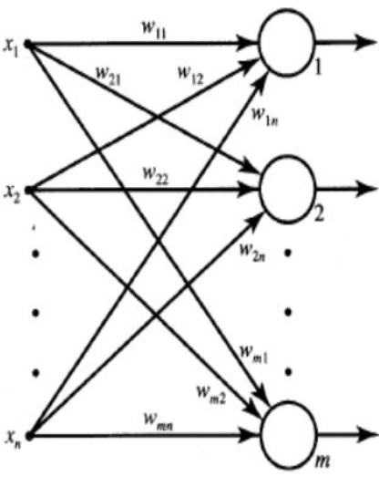
Make Classifier for all of the fashion images

How many inputs will the layer have?

How many outputs?

SciPy Perceptron

https://scikit-learn.org/stable/modules/generated/sklearn.linear_model.Perceptron.html

import numpy as np 
from sklearn.datasets import load_iris 
from sklearn.linear_model import Perceptron
iris = load_iris() 
X = iris.data[:, (2, 3)]  # petal length, petal width 
y = (iris.target == 0).astype(np.int)  # Iris Setosa?
per_clf = Perceptron(random_state=42) 
per_clf.fit(X, y)
y_pred = per_clf.predict([[2, 0.5]]) 

from matplotlib import pyplot as plt

a = -per_clf.coef_[0][0] / per_clf.coef_[0][1]
b = -per_clf.intercept_ / per_clf.coef_[0][1]

axes = [0, 5, 0, 2]

x0, x1 = np.meshgrid(
        np.linspace(axes[0], axes[1], 500).reshape(-1, 1),
        np.linspace(axes[2], axes[3], 200).reshape(-1, 1),
    )
X_new = np.c_[x0.ravel(), x1.ravel()]
y_predict = per_clf.predict(X_new)
zz = y_predict.reshape(x0.shape)

plt.figure(figsize=(10, 4))
plt.plot(X[y==0, 0], X[y==0, 1], "bs", label="Not Iris-Setosa")
plt.plot(X[y==1, 0], X[y==1, 1], "yo", label="Iris-Setosa")

plt.plot([axes[0], axes[1]], [a * axes[0] + b, a * axes[1] + b], "k-", linewidth=3)
from matplotlib.colors import ListedColormap
custom_cmap = ListedColormap(['#9898ff', '#fafab0'])

plt.contourf(x0, x1, zz, cmap=custom_cmap)
plt.xlabel("Petal length", fontsize=14)
plt.ylabel("Petal width", fontsize=14)
plt.legend(loc="lower right", fontsize=14)
plt.axis(axes)

plt.show()

Scikit-Learn’s Perceptron class is equivalent to using an SGDClassifier with the following hyperparameters:

• loss="perceptron",
• learning_rate="constant",
• eta0=1 (the learning rate),
• penalty=None (no regularization)

Note that contrary to Logistic Regression classifiers, Perceptrons do not output a class probability; rather, they just make predictions based on a hard threshold. This is one of the good reasons to prefer Logistic Regression over Perceptrons.

Alternative version of Layer

1. Make a layer of neurons with no activation functions (called a fully-connected layer)
2. Then make a layer of activation functions
3. Finally make composition function that applies one then other

Data Structures

Images, Signals, Vectors, and... Tensors

In a computer they are all just lists of numbers. We just need our code to handle them properly to perform the math we want.

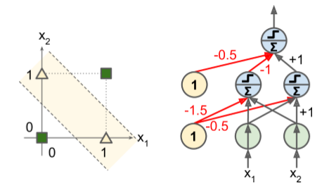
Problem: Non-linear Decision Boundaries

"Perceptrons", Marvin Minsky and Seymour Papert 1969

• highlighted a number of serious weaknesses of Perceptrons, in particular the fact that they are incapable of solving some trivial problems (e.g., the Exclusive OR (XOR) classification problem).
• true of any other linear classification model as well such as Logistic Regression classifiers),
• researchers had expected much more from Perceptrons, and their disappointment was great
• as a result, many researchers dropped connectionism altogether (i.e., the study of neural networks) in favor of higher-level problems such as logic, problem solving, and search.

Solution: Multilayer Perceptrons (LP)

• Some of the limitations of Perceptrons can be eliminated by stacking multiple Perceptrons.
• feed-forward: one-way flow of information
• The resulting ANN is called a Multi-Layer Perceptron (MLP)
• In particular, an MLP can solve the XOR problem

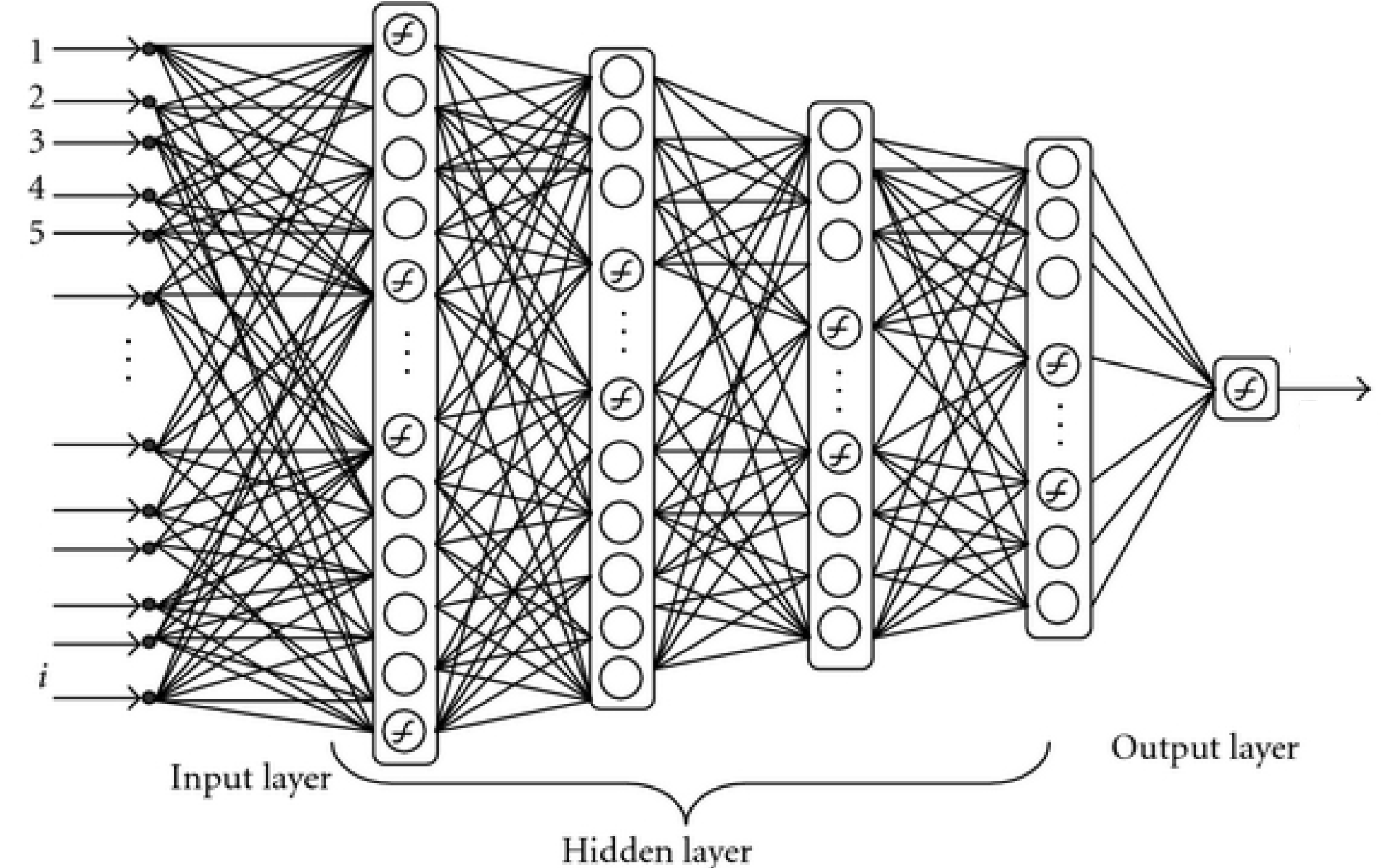
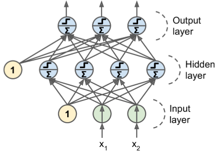
MLP Layers

An MLP is composed of

• one (passthrough) input layer,
• one or more layers of LTUs, called hidden layers,
• one final layer of LTUs called the output layer

Every layer except the output layer includes a bias neuron and is fully connected to the next layer.

When an ANN has two or more hidden layers, it is called a deep neural network (DNN).

Perceptron training algorithm doesn't extend to MLP's.

No good training algorithm for many years.

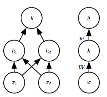
3. Make a Multi-layer Network with a Hidden Layer

Make a composition of layers and implement the XOR function from GBC as a single function call

Summing Up

So far we have:

1. Created networks as functions with adjustable weights
2. Applied a little learning algorithm to adjust the weights based on feeding one image at a time
3. Checked the accuracy of the result

Formal Machine Learning Framework & Jargon

1. Given training data $(\mathbf x_{(i)},y_i)$ for $i=1,...,m$.

2. Choose a model $f(\cdot)$ where we want to make $f(\mathbf x_{(i)})\approx y_i$ (for all $i$)

3. Define a loss function $L(f(\mathbf x), y)$ to minimize by changing $f(\cdot)$ ...by adjusting the weights.

Normally we don't implement the weight adjustment ourselves, we just tell the software what error metric to minimize.

Making a Deep Network in python

1. Make a function for a single neuron
2. Make function for a layer
3. Make a composition of layers