Deep Learning

Keith Dillon
Fall 2019

Topic 5: Neural Network Architectures

This topic:

1. Historic Architectures
2. Multilayer Perceptron

Reading:

• Geron Appendix E (Other Popular ANN Architectures)

I. Historic Network Architectures

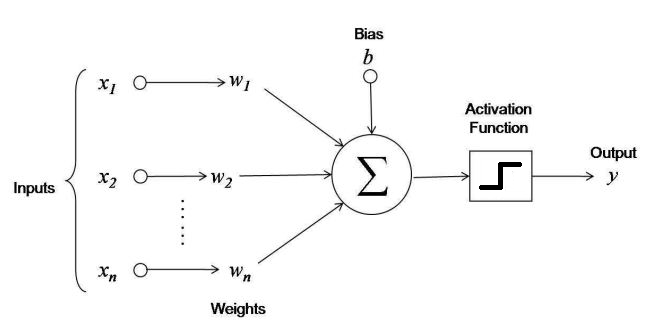
Fundamenal unit: the perceptron

• All artificial neural networks can be viewed as combinations of some kind of "perceptrons" in various architectures

• perhaps with small changes to the perceptron in terms of the activation function.

Key problem: Learning

A key to a given architecture's success (or lack thereof) is the existence of a training algorithm.

(also a lot of trial and error; other ideas may have been easy to train but just didn't work well)

Hopfield Networks

• first introduced by W. A. Little in 1974
• popularized by J. Hopfield in 1982
• associative memory networks
• useful in particular for character recognition

Hopfield Networks

• They are fully connected graphs - every neuron is connected to every other neuron.
• You first train the network by showing it examples of character images (each binary pixel maps to one neuron),
• then when you show it a new character image, after a few iterations it outputs the closest learned character.

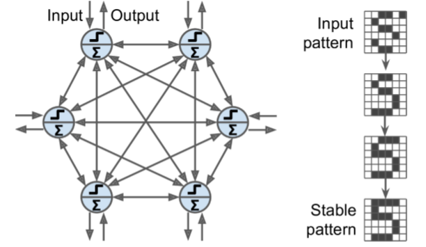
Note that on the diagram the images are 6 × 6 pixels, so the neural network on the left should contain 36 neurons (and 648 connections)

Hopfield Network Training

Hebb’s rule: for each training image, the weight between two neurons is increased if the corresponding pixels are both on or both off, but decreased if one pixel is on and the other is off.

• To show a new image to the network, you just activate the neurons that correspond to active pixels.
• The network then computes the output of every neuron, and this gives you a new image.
• You can then take this new image and repeat the whole process.
• After a while, the network reaches a stable state. Generally, this corresponds to the training image that most resembles the input image.

Energy function perspective of Hopfield nets

• At each iteration, the energy decreases, so the network is guaranteed to eventually stabilize to a low-energy state.
• The training algorithm tweaks the weights in a way that decreases the energy level of the training patterns, so the network is likely to stabilize in one of these lowenergy configurations.
• Unfortunately, some patterns that were not in the training set also end up with low energy, so the network sometimes stabilizes in a configuration that was not learned. These are called spurious patterns

Hopfield Network Capacity

• Memory capacity is roughly equal to 14% of the number of neurons.
• Example: to classify 28 × 28 images, you would need a Hopfield net with 784 fully connected neurons and 306,936 weights.
  • Such a network would only be able to learn about 110 different characters (14% of 784).
  • That’s a lot of parameters for such a small memory.
• Hence Hopfield nets don’t scale very well

Boltzmann Machines

• Invented in 1985 by Geoffrey Hinton and Terrence Sejnowski.
• Also fully connected ANNs,
• Stochastic neurons: instead of using a deterministic step function to decide what value to output, these neurons output 1 with some probability, and 0 otherwise.
• The probability function that these ANNs use is based on the Boltzmann distribution from statistical mechanics
  • $p(s_i=1) = \sigma(\frac{1}{T}[\sum w_j s_j + b_i])$, $s_i$ is state of $i$th neuron.
  • Temperatue $T$ sets degree of randomness.

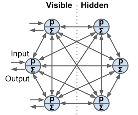
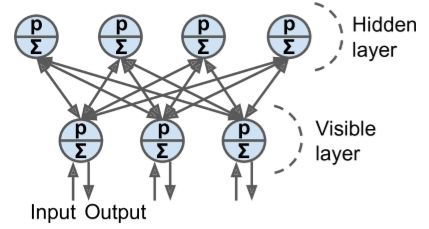
Neurons separated into two groups: visible units (receive inputs and produce outputs) and hidden units

Boltzmann machine as a Generative model

• Boltzmann machine will never stabilize into a fixed configuration, but instead it will keep switching between many configurations
• ultimately, the probability of observing a particular configuration (out of the many states it continually switches among) will only be a function of the connection weights and bias terms, not of the original configuration
  • similarly, after you shuffle a deck of cards for long enough, the configuration of the deck does not depend on the initial state
  • known as thermal equilibrium
• By setting the network parameters appropriately, letting the network reach thermal equilibrium, and then observing its state, we can simulate a wide range of probability distributions $\rightarrow$ a generative model.

Training a Boltzmann machine

• finding the parameters that will make the network approximate the training set’s probability distribution.
• Example: if there are three visible neurons and the training set contains 75% (0, 1, 1) triplets, 10% (0, 0, 1) triplets, and 15% (1, 1, 1) triplets, then after training a Boltzmann machine, you could use it to generate random binary triplets with about the same probability distribution. About 75% of the time it would output the (0, 1, 1) triplet.
• No efficient method to do this training

Boltzmann Machine Applications

Image correction/denoising

• if it is trained on images, and you provide an incomplete or noisy image to the network, it will automatically “repair” the image in a reasonable way.

Generative model for classification.

• Add a few visible neurons to encode the training image’s class (e.g., add 10 visible neurons and turn on only the fifth neuron when the training image represents a 5).
• Then, when given a new image, the network will automatically turn on the appropriate visible neurons, indicating the image’s class (e.g., it will turn on the fifth visible neuron if the image represents a 5).

Restricted Boltzmann Machines (RBM)

A Boltzmann machine in which there are no connections between visible units or between hidden units, only between visible and hidden units

RBM Training - Contrastive Divergence

A very efficient training algorithm introduced in 2005 by Miguel Á. Carreira-Perpiñán and Geoffrey Hinton.

1. for each training instance $\mathbf x$, the algorithm starts by feeding it to the network by setting the state of the visible units to $x_1, x_2, ⋯, x_n$.
2. Then you compute the state of the hidden units by applying the stochastic equation
3. This gives you a hidden vector $\mathbf h$ (where $h_i$ is equal to the state of the $i$th unit).
4. Next you compute the state of the visible units, by applying the same stochastic equation.
5. This gives you a vector $\dot{\mathbf x}$
6. Then once again you compute the state of the hidden units, which gives you a vector $\dot{\mathbf h}$˙
7. Now you can update each connection weight by applying the rule

$$ w_{ij} = w_{ij} + \eta (\mathbf x \mathbf h^T - \dot{\mathbf x}\dot{\mathbf h}^T) $$

• does not require waiting for the network to reach thermal equilibrium
• it just goes forward, backward, and forward again, and that’s it.
• This makes it incomparably more efficient than previous algorithms
• was a key ingredient to the first success of Deep Learning based on multiple stacked RBMs.

Deep Belief Nets

• Stack of RBMs - the hidden units of the first-level RBM serves as the visible units for the second-layer RBM, and so on.
• Yee-Whye Teh, one of Geoffrey Hinton’s students, observed that it was possible to train DBNs one layer at a time using Contrastive Divergence, starting with the lower layers and then gradually moving up to the top layers.
• This led to the groundbreaking article that kickstarted the Deep Learning tsunami in 2006
• Were the state of the art in Deep Learning until the early 2010s
• still the subject of very active research

DBNs as Hierarchical Generative models

• Just like RBMs, DBNs learn to reproduce the probability distribution of their inputs, without any supervision.
• they are much better at it, for the same reason that deep neural networks are more powerful than shallow ones
• real-world data is often organized in hierarchical patterns, and DBNs take advantage of that.
• Their lower layers learn low-level features in the input data, while higher layers learn high-level features.

Supervised Learning with DBNs

• Just like RBMs, DBNs are fundamentally unsupervised,
• But can also train them in a supervised manner by adding some visible units to represent the labels.

Combine data with labels as inputs to first RBM

Semi-supervised Learning

Motivation - a baby

• learns to recognize objects without supervision,
• so when you point to a chair and say “chair,” the baby can associate the word “chair” with the class of objects it has already learned to recognize on its own.
• You don’t need to point to every single chair and say “chair”; only a few examples will suffice (just enough so the baby can be sure that you are indeed referring to the chair, not to its color or one of the chair’s parts).

Benefit of semi-supervised approach is that you don’t need much labeled training data.

If the unsupervised RBMs do a good enough job, then only a small amount of labeled training instances per class will be necessary.

Semi-supervised Learning Architecture

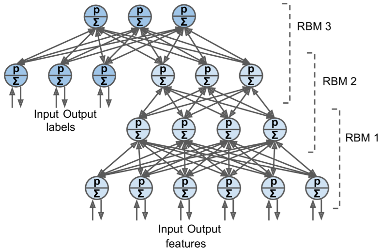
1. RBM 1 is trained without supervision. It learns low-level features in the training data.
2. RBM 2 is trained with RBM 1’s hidden units as inputs, again without supervision:
   • it learns higher-level features
   • note that RBM 2’s hidden units include only the three rightmost units, not the label units
   • Several more RBMs could be stacked this way
3. RBM 3 is trained using both RBM 2’s hidden units as inputs, as well as extra visible units used to represent the target labels
   • e.g., a one-hot vector representing the instance class
   • It learns to associate high-level features with training labels.
   • This is the supervised step.

Classification of a new sample

1. feed RBM 1 a new instance,
2. the signal will propagate up to RBM 2,
3. then up to the top of RBM 3, and
4. then back down to the label units;
5. hopefully, the appropriate label will light up

DBN in Reverse

• If you activate one of the label units, the signal will propagate up to the hidden units of RBM 3,
• then down to RBM 2,
• then RBM 1,
• and a new instance will be output by the visible units of RBM 1.

This new instance will usually look like a regular instance of the class whose label unit you activated.

Applications

• Automatically generate captions for images
• Automatically generate example images given captions

1. first a DBN is trained (without supervision) to learn features in images,
2. another DBN is trained (again without supervision) to learn features in sets of captions (e.g., “car” often comes with “automobile”).
3. Then an RBM is stacked on top of both DBNs and trained with a set of images along with their captions; it learns to associate high-level features in images with high-level features in captions.
4. Next, if you feed the image DBN an image of a car, the signal will propagate through the network, up to the top-level RBM, and back down to the bottom of the caption DBN, producing a caption.

Due to the stochastic nature of RBMs and DBNs, the caption will keep changing randomly, but it will generally be appropriate for the image. If you generate a few hundred captions, the most frequently generated ones will likely be a good description of the image.

Self-Organizing Maps

• used to produce a low-dimensional representation of a high-dimensional dataset,

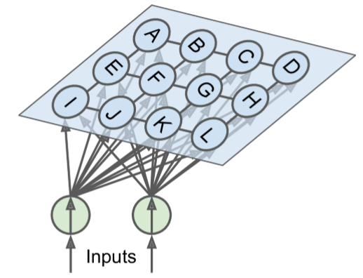
• The neurons are spread across a map (typically 2D for visualization
• Each neuron has a weighted connection to every input (note that the diagram shows just two inputs, but there are typically a very large number)
• Once the network is trained, you can feed it a new instance and this will activate only one neuron (i.e., hence one point on the map): the neuron whose weight vector is closest to the input vector

Applications

• Visualization/clustering - can identify clusters of data based on neuron clusters
• Classification - choose regions (via another method) which select for input class

SOM Training

unsupervised - works by having all the neurons compete against each other.

1. weights are initialized randomly.
2. a training instance is picked randomly and fed to the network.
3. All neurons compute the distance between their weight vector and the input vector (this is very different from the artificial neurons we have seen so far).
4. The neuron that measures the smallest distance wins and tweaks its weight vector to be even slightly closer to the input vector, making it more likely to win future competitions for other inputs similar to this one.
5. It also recruits its neighboring neurons, and they too update their weight vector to be slightly closer to the input vector (but they don’t update their weights as much as the winner neuron).
6. Then the algorithm picks another training instance and repeats the process, again and again.

This algorithm tends to make nearby neurons gradually specialize in similar inputs

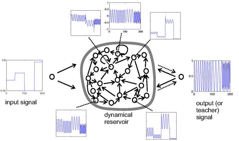
Liquid state Machines

Use random network to generate a collection of pseudorandom sequences

Use regression layer at output to form desired waveform by linear combination

II. MultiLayer Perceptrons

Most popular Network Architectures

• Deep Multi-Layer Perceptrons
• Convolutional neural networks
• Recurrent neural networks
• Autoencoders

All can be viewed as combinations of "perceptrons" in networks, perhaps with small changes to the perceptron in terms of the activation function.

A key to their success is the existence of a training algorithm.

(also a lot of trial and error; other ideas may have been easy to train but just didn't work well)

A "Layer" of neurons

What are the inputs and outputs?

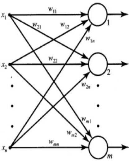
How might you use this for multi-class classification?

Layers

• A Layer basically means there are Multiple outputs via mutiple nodes
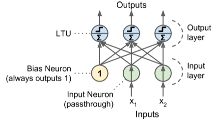
• A Perceptron is simply composed of a single layer of LTUs
• with each neuron connected to all the inputs.
• These connections are often represented using special pass-through neurons called input neurons: they just output whatever input they are fed.
• Moreover, an extra bias feature is generally added ($x_0 = 1$). This bias feature is typically represented using a special type of neuron called a bias neuron, which just outputs 1 all the time

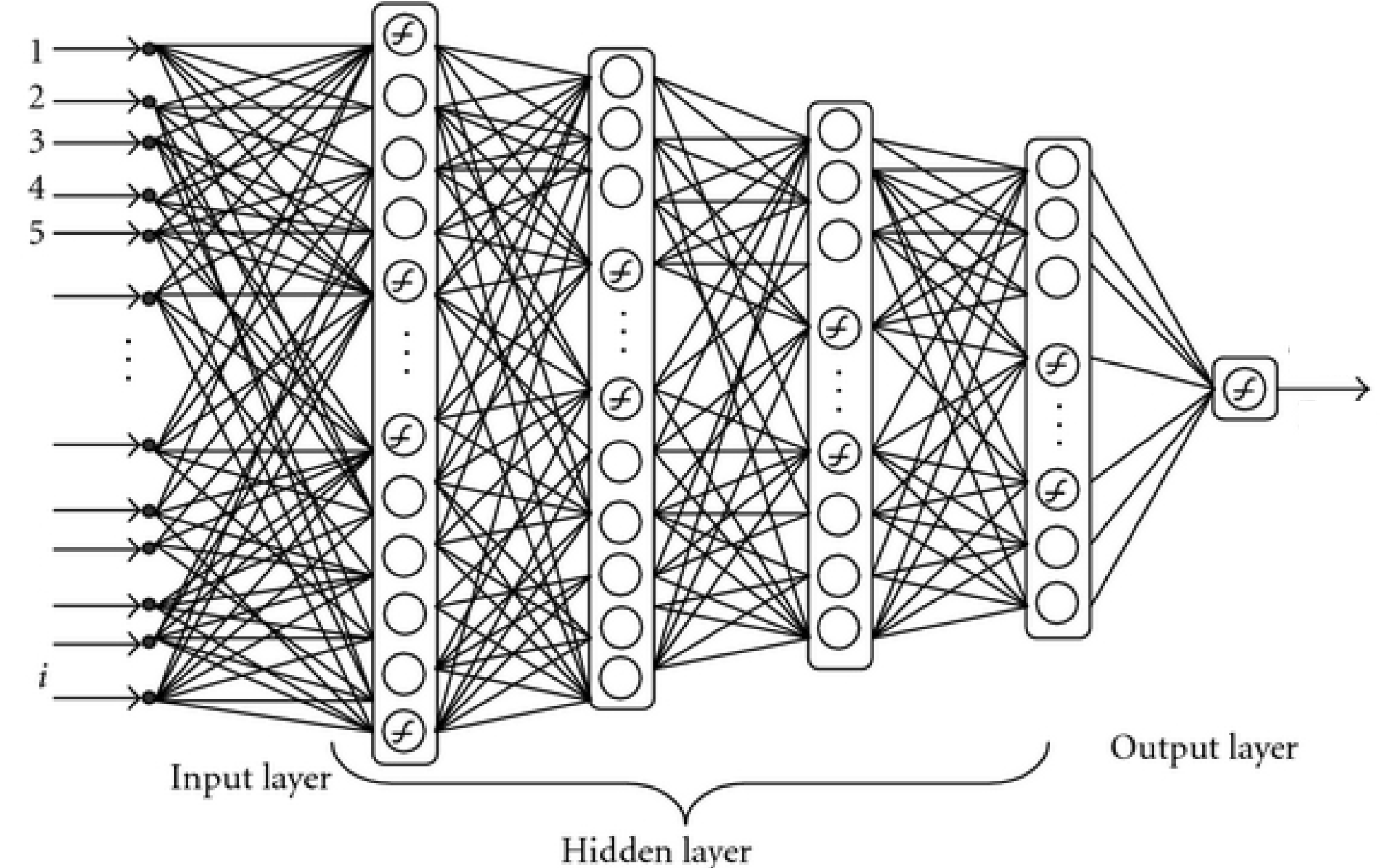
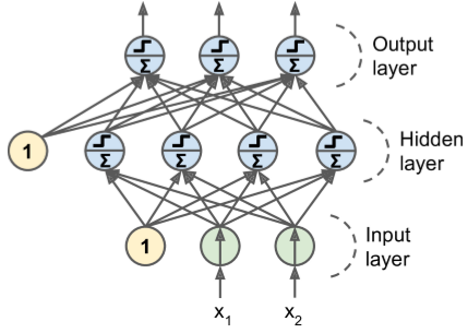
MLP Layers

An MLP is composed of

• one (passthrough) input layer,
• one or more layers of LTUs, called hidden layers,
• one final layer of LTUs called the output layer

Every layer except the output layer includes a bias neuron and is fully connected to the next layer.

When an ANN has two or more hidden layers, it is called a deep neural network (DNN).

Perceptron training algorithm doesn't extend to MLP's.

No good training algorithm for many years.

"Deep (feedforward) network"

A series of layers