Deep Learning
Keith Dillon
Spring 2019
Topic 8: Keras
Today:
- Keras Quick Overview & Demo
- Implementing MLP's in Keras
- Normalizing data
- Comparing Keras MLP with ours
- Multi-category classifier in Keras
Reading:
- Chollet Chapter 1
- Chollet: Chapter 4
- GBC: Chapter 8
- "Getting Started with TensorFlow and Deep Learning: SciPy 2018 Tutorial", Josh Gordon, https://www.youtube.com/watch?v=tYYVSEHq-io, https://www.tensorflow.org/tutorials/keras/

$\bf x$ - input data ~ a single image, or sentence of text.
$\bf y$ - prediction ~ "cat" vs "dog", "positive" vs "negative"
$f(\cdot)$ - mapping from input to output - function we fit
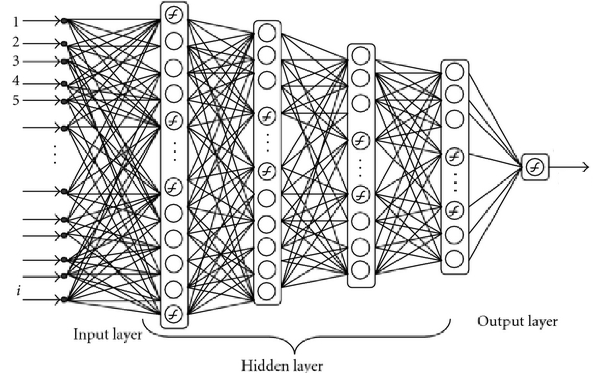
Layers in Keras
Connection decisions: Fully-connected Layers, Convolutional Layers
Unified way to define other aspects of network: activation function, dropout, even pre-processing steps
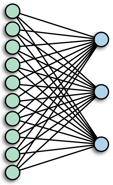
Fully-connected Layer
a.k.a. Densely-connected Layer - every input connects to every output (with weights)
Formal Machine Learning Framework & Jargon
Given training data $(\mathbf x_{(i)},y_i)$ for $i=1,...,m$.
Choose a model $f(\cdot)$ where we want to make $f(\mathbf x_{(i)})\approx y_i$ (for all $i$)
Define a loss function $L(f(\mathbf x), y)$ to minimize by changing $f(\cdot)$ ...by adjusting the weights.
Deep Network Design
Make up an architcture - choose layers and their parameters
Choose a Loss function - how compute error for $f(\mathbf x_{(i)}) \ne y_i$
Choose a optimization method - many variants of same basic method
Choose "regularization" tricks to prevent overfitting
Other important details like initializing and normalizing data
Keras example
"Deep Learning with Python", Francois Chollet, Ch. 2,
Train your first neural network: basic classification
This tutorial is an updated version of code from book:
- https://www.tensorflow.org/tutorials/keras/basic_classification
- https://github.com/tensorflow/docs/blob/master/site/en/tutorials/keras/basic_classification.ipynb
Variation on the Chollet version in the following...
# TensorFlow
import tensorflow as tf

print(tf.__version__)
import keras
keras.__version__
The Data
Look at the data and understand the structure
fashion_mnist = keras.datasets.fashion_mnist

(train_images, train_labels), (test_images, test_labels) = fashion_mnist.load_data()
class_names = ['T-shirt/top', 'Trouser', 'Pullover', 'Dress', 'Coat',
               'Sandal', 'Shirt', 'Sneaker', 'Bag', 'Ankle boot']

print(train_images.shape)
print(test_images.shape)
print(train_labels)
"Preprocessing"
Pixel values commonly range from 0 to 255 (8 bit integers)
We want to normalize to between 0 and 1
pixel0 = train_images[0][0][0]

print(pixel0)
plt.imshow(train_images[0])
plt.colorbar();

train_images[0]
plt.plot(train_images[0]);

Normalizing
train_images = train_images / 255.0
test_images = test_images / 255.0
plt.imshow(train_images[0])
plt.colorbar();

plt.figure(figsize=(10,10))
for i in range(25):
    plt.subplot(5,5,i+1)
    plt.xticks([])
    plt.yticks([])
    plt.grid(False)
    plt.imshow(train_images[i], cmap=plt.cm.binary)
    plt.xlabel(class_names[train_labels[i]])

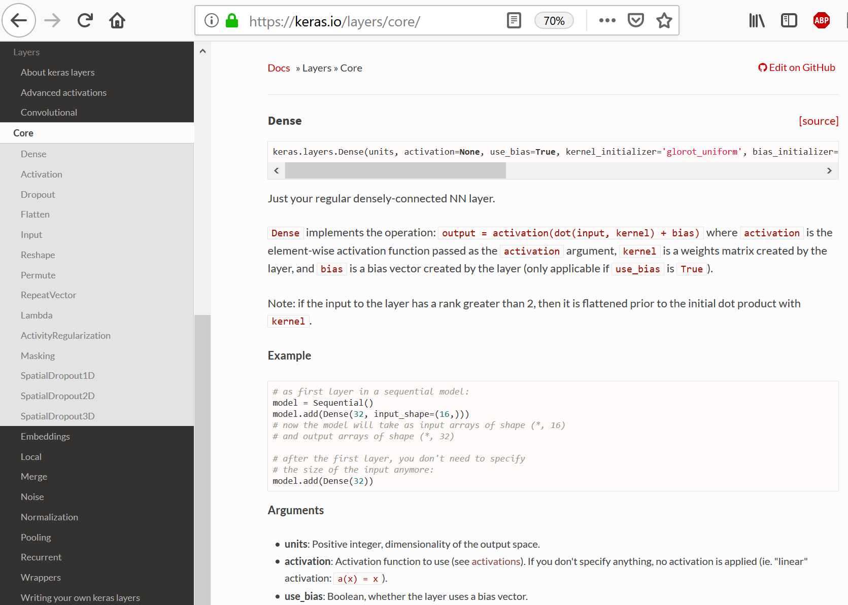
Define the network model
from keras import models
from keras import layers

model = models.Sequential() # model as a list (sequence) of layers
model.add(layers.Flatten(input_shape=(28, 28)))
model.add(layers.Dense(128, activation=tf.nn.relu))
model.add(layers.Dense(32, activation=tf.nn.relu))
model.add(layers.Dense(10, activation=tf.nn.softmax))
model.summary()
"Compile" the network
model.compile(optimizer=tf.train.AdamOptimizer(),
              loss='sparse_categorical_crossentropy',
              metrics=['accuracy'])
- Sparse - recall what this means?
- Cross-entropy
- Categorical Cross-entropy
Optimize the network
I.e. change weights in $f(\cdot)$ such that $f(\mathbf x) \approx y$, using training set
model.fit(train_images, train_labels, epochs=5)
Compute accuracy on test set
test_loss, test_acc = model.evaluate(test_images, test_labels)

print('Test accuracy:', test_acc)
Use network to classify samples - compute $y = f(\mathbf x)$
predictions = model.predict(test_images)
plt.plot(predictions[3]);

print(np.argmax(predictions[0]), test_labels[0])
print("Prediction:",class_names[np.argmax(predictions[0])], "vs. Truth:",class_names[test_labels[0]])
Note: .predict() expects an array of samples (as a tensor)
img = test_images[0]

print(img.shape)
img_tensor = (np.expand_dims(img,0))

print(img_tensor.shape)
predictions_single = model.predict(img_tensor)

print(predictions_single)
predictions_single = model.predict(np.array([img]))

print(predictions_single)
II. Part 2...
Normalizing data
from sklearn.datasets import load_breast_cancer
bcdata = load_breast_cancer()

X=bcdata.data
y=bcdata.target
#print(X.shape,y.shape,y)
print(X[0])
np.linalg.norm(keras.utils.normalize([[1,2,3],[2,3,4]],axis=0)[:,0])
Formal Machine Learning Framework & Jargon
Given training data $(\mathbf x_{(i)},y_i)$ for $i=1,...,m$.
Choose a model $f(\cdot)$ where we want to make $f(\mathbf x_{(i)})\approx y_i$ (for all $i$)
Define a loss function $L(f(\mathbf x), y)$ to minimize by changing $f(\cdot)$ ...by adjusting the weights.
In Keras
Make up an architecture - choose layers and their parameters
Choose a Loss function - how compute error for $f(\mathbf x_{(i)}) \ne y_i$
Choose a optimization method - many variants of same basic method
Choose "regularization" tricks to prevent overfitting
Handle other important details like initializing and normalizing data
Perceptron in Keras
Redo the single class predictor using Keras for the breast cancer data.
Use the sequential model in Keras and make a single neuron. https://keras.io/getting-started/sequential-model-guide/
# load dataset, "preprocess"

from sklearn.datasets import load_breast_cancer
bcdata = load_breast_cancer()

X=bcdata.data
y=bcdata.target
#print(X.shape,y.shape,y)
print(X[0])
print(bcdata.feature_names)
test_loss, test_acc = perceptron1.evaluate(X, y)

print('Test accuracy:', test_acc)
Comparing with our Perceptron
perceptron1.get_weights()
Use weights and bias from Keras in our python program
w = perceptron1.get_weights()[0]
w.shape
b = perceptron1.get_weights()[1][0]
b
def f(x,w,b):
    sum = 0
    for i in range(0,len(w)):
        sum = sum+x[i]*w[i]
        #print(x[i],w[i],sum)
    return activation(sum+b)

def activation(y_0):
    if y_0 >= 0:
        return 1
    else:
        return 0 # <----- using zero
Our network:
acc = 0
for j in np.arange(0,len(X)):
    acc = acc + (y[j]==f(X[j].reshape(-1),w,b))/len(X);
print(acc)
Keras network:
test_loss, test_acc = perceptron1.evaluate(X, y)

print('Test accuracy:', test_acc)
...perfect!
Multi-category classification
Iris Dataset
https://scikit-learn.org/stable/modules/generated/sklearn.datasets.load_iris.html
# load dataset

from sklearn import datasets
iris = datasets.load_iris()
X=iris.data
from keras.utils import to_categorical
y = to_categorical(iris.target)

print(X.shape,y.shape)

X = 2*X*(1/np.max(np.abs(X),0))-1 # normalize
print(np.max(X,0),np.min(X,0))
y
perceptron2.fit(X, y, epochs = 100, batch_size = 12, shuffle = True)
test_loss, test_acc = perceptron2.evaluate(X, y)

print('Test accuracy:', test_acc)