Outline:
- Convolution
- Convolutional layers
- Pooling Layers
- Keras CNN
- Using a pre-optimized model
Reading:
- Chollet Chapter 5
- GBC 9.0,9.1,9.2,9.3,9.10,9.11
- "A guide to convolution arithmetic for deep learning", https://arxiv.org/pdf/1603.07285.pdf
CNN's
- "perhaps the greatest success story of biologically-inspired artificial intelligence" -GBC
- ImageNet 2012 challenge (and computer visions competitions since).
- Best approach for many major computer vision tasks.
- Applied to text, speech signals, and other data types also.
Inspiration - Computer vision
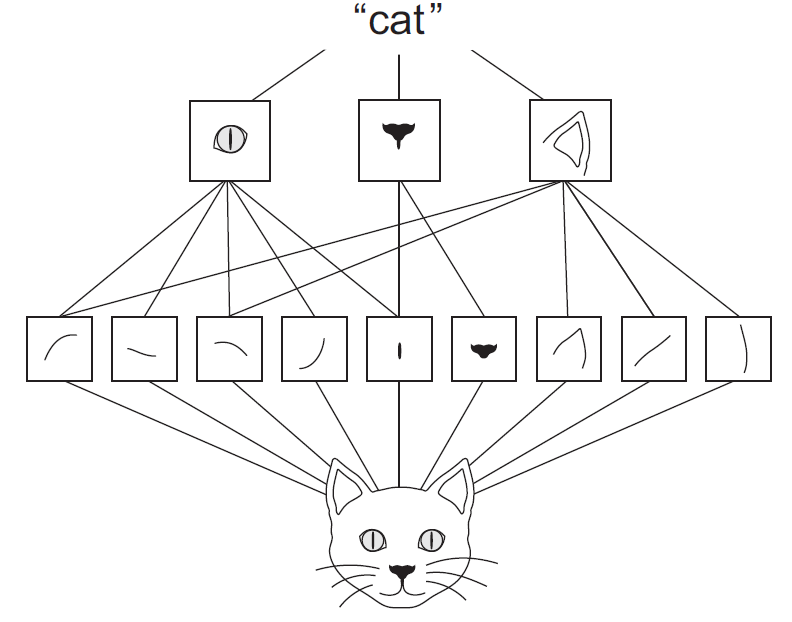
Note the features can be anywhere in image, hence "unstructured".
Biological inspiration - the Receptive Field
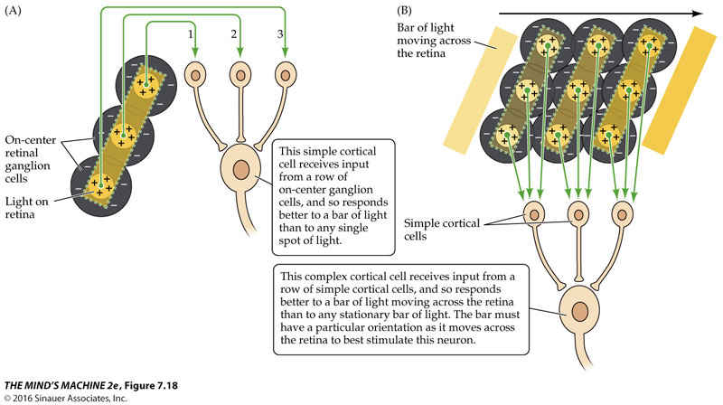
"Center-surround" fields at every point in visual field
Can implement via 2D convolution
Combine in subsequent neurons to make more sophisticated receptive fields.
Convolution
A "sliding dot product": \begin{align} s[i] &= \sum_{n=-\infty}^\infty x[n] w[i-n] = (x * w)(i) \end{align} Compare to \begin{align} s'[i] &= \sum_{n=-\infty}^\infty x[n] w[i+n] = (x \star w)(i) \end{align}
Exercise: Compute convolution of w = [-1, +1, -1] with:
- x = [1, 2, 3, 4, 6, 7, 7, 6]
- x = [0, 0, 0, -1, +1, -1, 0]
for $i$=0, 1, ..., $N$
How might you deal with the edges?
What do the following convolution kernels do?
- w=[1,1,1]
- w=[-1, +1]
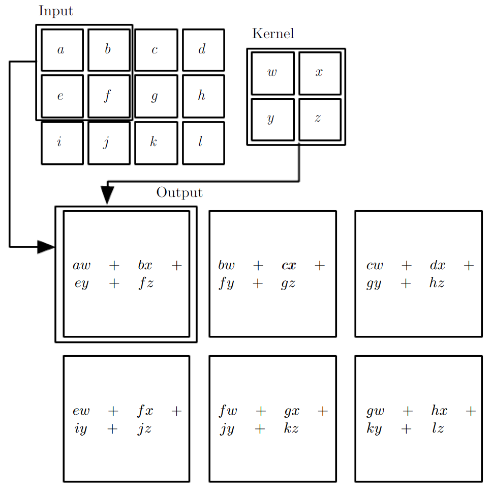
2D Convolution
\begin{align} s[i,j] &= \sum_{m=0}^M\sum_{n=0}^N x[m,n] w[i-m][j-n] = (x * w)(i,j) \\ s'[i,j] &= \sum_{m=0}^M\sum_{n=0}^N x[m,n] w[i+m][j+n] = (x \star w)(i,j) \\ \end{align}Recall sliding dot product $\rightarrow$ pattern matching
Some enlightening gifs found on internet: https://towardsdatascience.com/intuitively-understanding-convolutions-for-deep-learning-1f6f42faee1
Q: How do we implement Convolution as a network layer?
Recall fully-connected a.k.a. Densely-connected a.k.a dense Layer
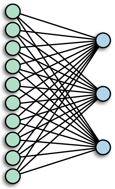
Suppose input was an image, and output is an image (with convolution applied). Apply equation: \begin{align} s[i] &= \sum_{n=0}^N x[n] w[i-n] = (x * w)(i) \end{align}
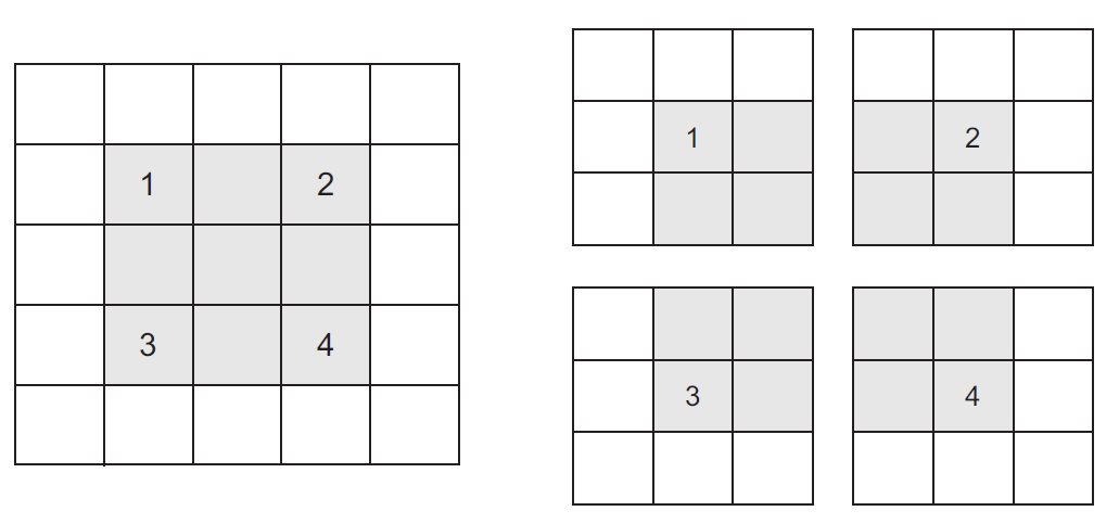
Convolutional Layer
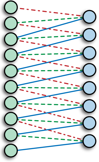
Parameter sharing (same color = same weight)
Far fewer weights to deal with versus dense layer.
Also note how edges handled ~ image gets smaller.
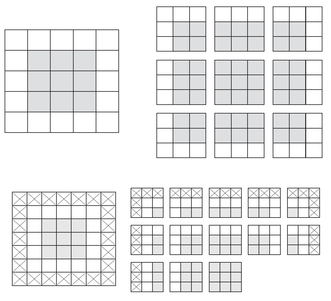
Edge handling
Two options:
- Edges thrown away, each layer gets smaller
- Must pad image (which then shrinks back to original size)
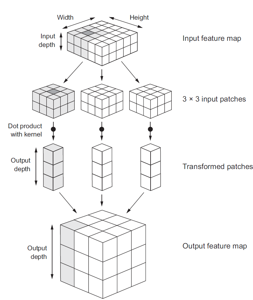
Multiple Channels & Kernels
We know how to make a 2D image into a 1D vector (right?). What is a color image however?
We can also have multiple convolution kernels for the same input image
Biological inspiration II
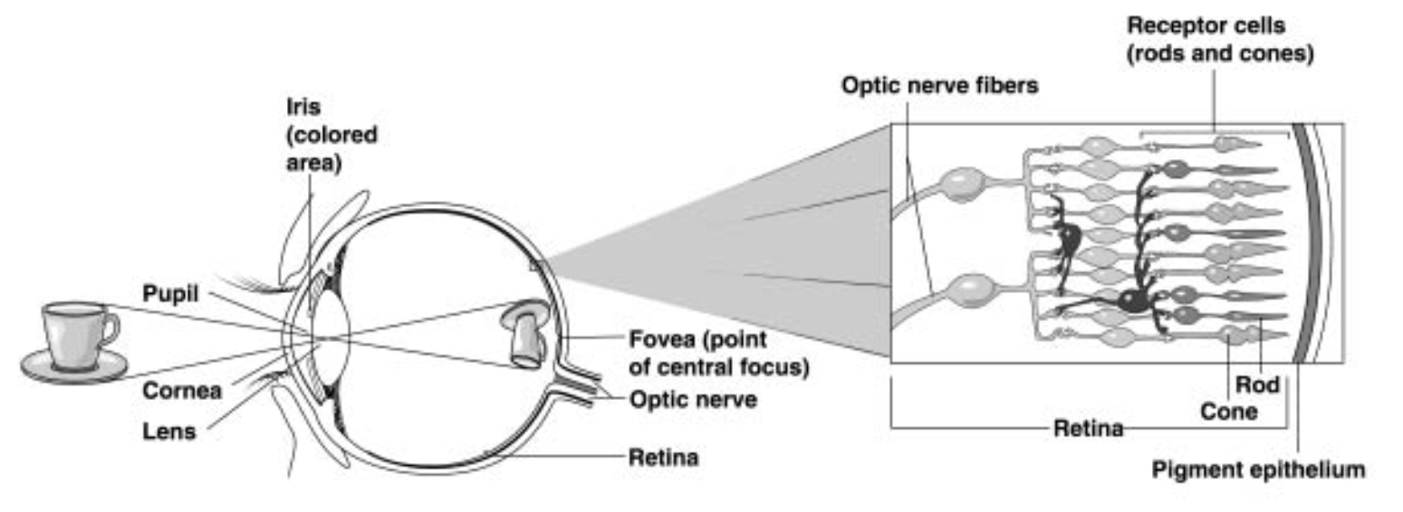
- Retina $\approx$ 100 million photoreceptors
- Optic nerve $\approx$ 1 million axons
100x downsampling.
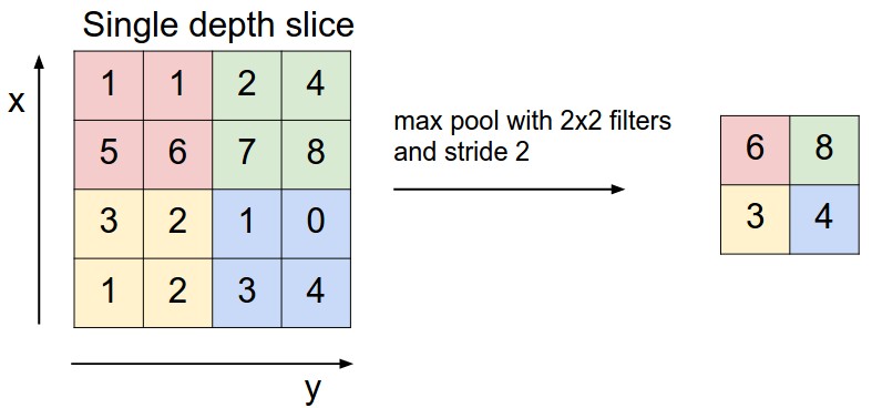
Pooling Layer
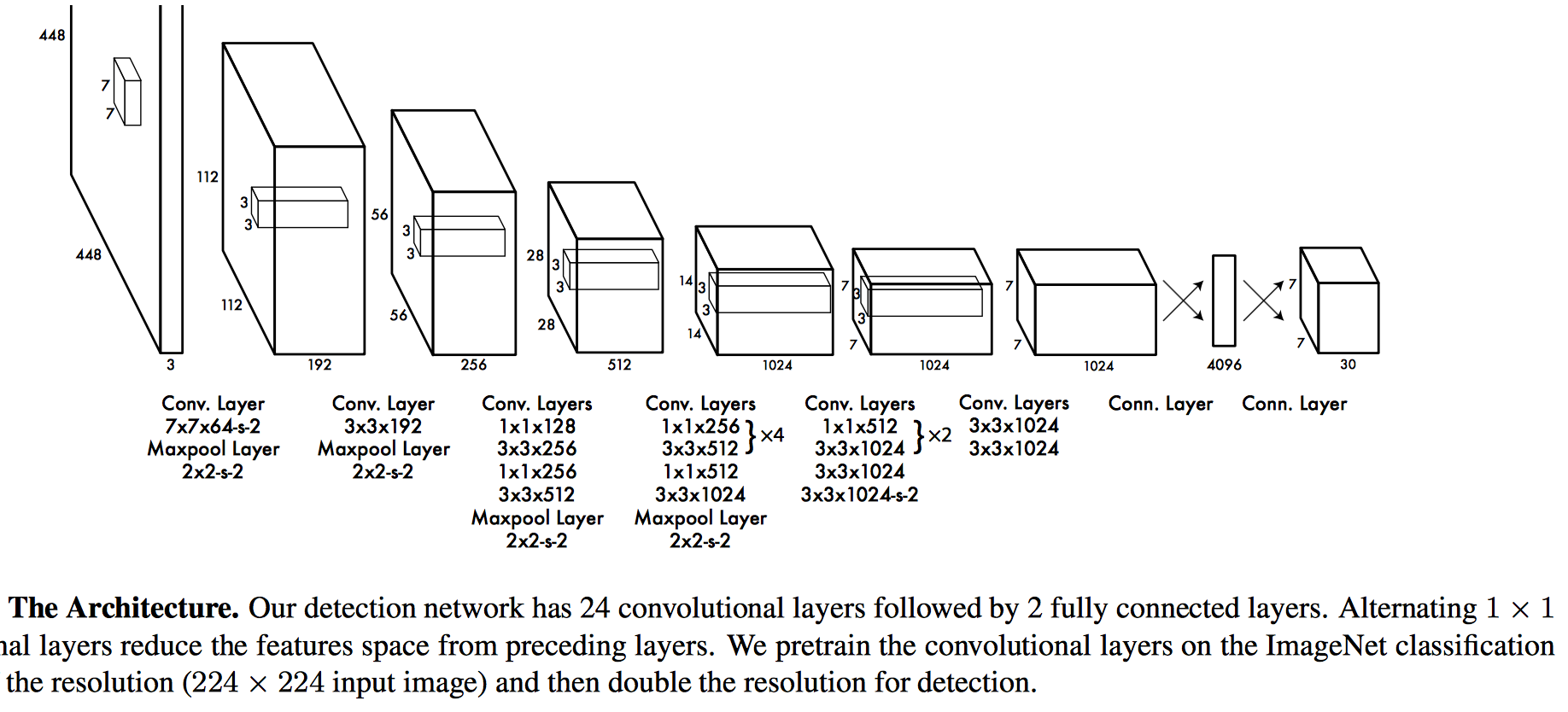
Combining everything...
Keras time
"Deep Learning with Python", Francois Chollet, Ch. 2, https://github.com/fchollet/deep-learning-with-python-notebooks
"Getting Started with TensorFlow and Deep Learning: SciPy 2018 Tutorial", Josh Gordon, https://www.youtube.com/watch?v=tYYVSEHq-io, https://www.tensorflow.org/tutorials/keras/
Classification demos
https://www.tensorflow.org/tutorials/keras/basic_classification
https://github.com/tensorflow/docs/blob/master/site/en/tutorials/keras/basic_classification.ipynb
First test a Dense network on the fashion MNIST dataset
mnist = keras.datasets.mnist

(X_train, y_train), (X_test, y_test) = mnist.load_data()
print(X_train.shape)
print(X_test.shape)
print(y_train)
showMNIST10x10()

"Preprocessing"
Note pixel values range from 0 to 255 (8 bit integers)
We want to "normalize" to between 0 and 1
plt.imshow(X_train[0])
plt.colorbar();

X_train = X_train / 255.0
X_test = X_test / 255.0
Dense network model
from keras import models
from keras import layers

model = models.Sequential()
model.add(layers.Flatten(input_shape=(28, 28)))
model.add(layers.Dense(128, activation=tf.nn.relu))
model.add(layers.Dense(10, activation=tf.nn.softmax))

model.summary()
model.compile(optimizer=tf.train.AdamOptimizer(),
              loss='categorical_crossentropy',
              metrics=['accuracy'])
from keras.utils import to_categorical
y_train_cat = to_categorical(y_train)

model.fit(X_train, y_train_cat, epochs=5)
y_test_cat = to_categorical(y_test)
test_loss, test_acc = model.evaluate(X_test, y_test_cat)

print('Test accuracy:', test_acc)
Using Validation data
from sklearn.model_selection import train_test_split

X_test, X_valid, y_test, y_valid = train_test_split(X_test, y_test, test_size=0.33)

from keras.utils import to_categorical
y_test_cat = to_categorical(y_test)
y_valid_cat = to_categorical(y_valid)
model = models.Sequential()
model.add(layers.Flatten(input_shape=(28, 28)))
model.add(layers.Dense(128, activation=tf.nn.relu))
model.add(layers.Dense(10, activation=tf.nn.softmax))

model.compile(optimizer=tf.train.AdamOptimizer(),
              loss='categorical_crossentropy',
              metrics=['accuracy'])

history =  model.fit(X_train, y_train_cat, validation_data=(X_valid,y_valid_cat), epochs=20)
acc = history.history['acc']
val_acc = history.history['val_acc']
loss = history.history['loss']
val_loss = history.history['val_loss']
epochs = range(len(acc))

plt.plot(epochs, acc, 'bo', label='Training acc')
plt.plot(epochs, val_acc, 'b', label='Validation acc')
plt.title('Training and validation accuracy')
plt.legend();

plt.figure()

plt.plot(epochs, loss, 'bo', label='Training loss')
plt.plot(epochs, val_loss, 'b', label='Validation loss')
plt.title('Training and validation loss')
plt.legend();

...what are these plots telling us?
Now use Convolutional and max-pooling layers
# reload and normalize the data for clarity

mnist = keras.datasets.mnist

(X_train, y_train), (X_test, y_test) = mnist.load_data()

X_train = X_train / 255.0
X_test = X_test / 255.0

# note new step needed - convolutional layers expect channel dimension
X_train = X_train.reshape((60000, 28, 28, 1))
X_test = X_test.reshape((10000, 28, 28, 1))

from sklearn.model_selection import train_test_split
X_test, X_valid, y_test, y_valid = train_test_split(X_test, y_test, test_size=0.33)

from keras.utils import to_categorical
y_train_cat = to_categorical(y_train)
y_test_cat  = to_categorical(y_test)
y_valid_cat = to_categorical(y_valid)
from keras import layers
from keras import models

model = models.Sequential()
model.add(layers.Conv2D(32, (3, 3), activation='relu', input_shape=(28, 28, 1)))
model.add(layers.MaxPooling2D((2, 2)))
model.add(layers.Conv2D(64, (3, 3), activation='relu'))
model.add(layers.Flatten())
model.add(layers.Dense(64, activation='relu'))
model.add(layers.Dense(10, activation='softmax'))
model.summary()
model.compile(optimizer=tf.train.AdamOptimizer(),
              loss='categorical_crossentropy',
              metrics=['accuracy'])

history =  model.fit(X_train, y_train_cat, validation_data=(X_valid,y_valid_cat), epochs=20)
model.save('myCNN1.h5')
acc = history.history['acc']
val_acc = history.history['val_acc']
loss = history.history['loss']
val_loss = history.history['val_loss']
epochs = range(len(acc))

plt.plot(epochs, acc, 'bo', label='Training acc')
plt.plot(epochs, val_acc, 'b', label='Validation acc')
plt.title('Training and validation accuracy')
plt.legend();

test_loss, test_acc = model.evaluate(X_test, y_test_cat)
test_acc
Using pre-optimized models
As you can see, convolutional networks perform quite a bit better than dense networks, but also much slower.
The real power becomes evident when trained on huge datasets, which also allow much deeper networks to be optimized without overfitting (too much).
However this requires significant supercomputing resources and days to weeks of time to optimize.
Rather than optimize a network from scratch however, we can load a pre-optimized network to use.