Outline:
- Sequence data
- Text data
- Recurrent Neural Networks
Reading:
- Chollet Chapter 6
- GBC Chapter 10 (advanced)
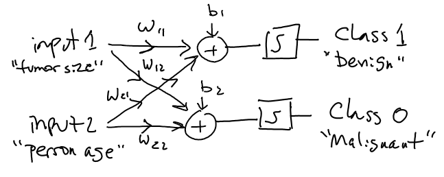
Recall: Structured Data ~ Features & Samples
With structured data, we had vectors of information for each sample (i.e. $\mathbf x^{(k)}$). The position in the vector is meaningful, e.g., size of tumor, or flower petal length, or individual's height.
Neural networks handle this perfectly, because the input with the same meaning always can be fed into the same input node.
Recall: Image Data ~ pixels
Generally called "unstructured data", but actually have very important structure. Pixel location has real-world meaning.
Neighboring pixels are related in horizontal and vertical directions. The three color channels for a pixel are related.
So rather than simply convert pixels into a vector, they are handled directly as images (actually tensors) throughout the network.
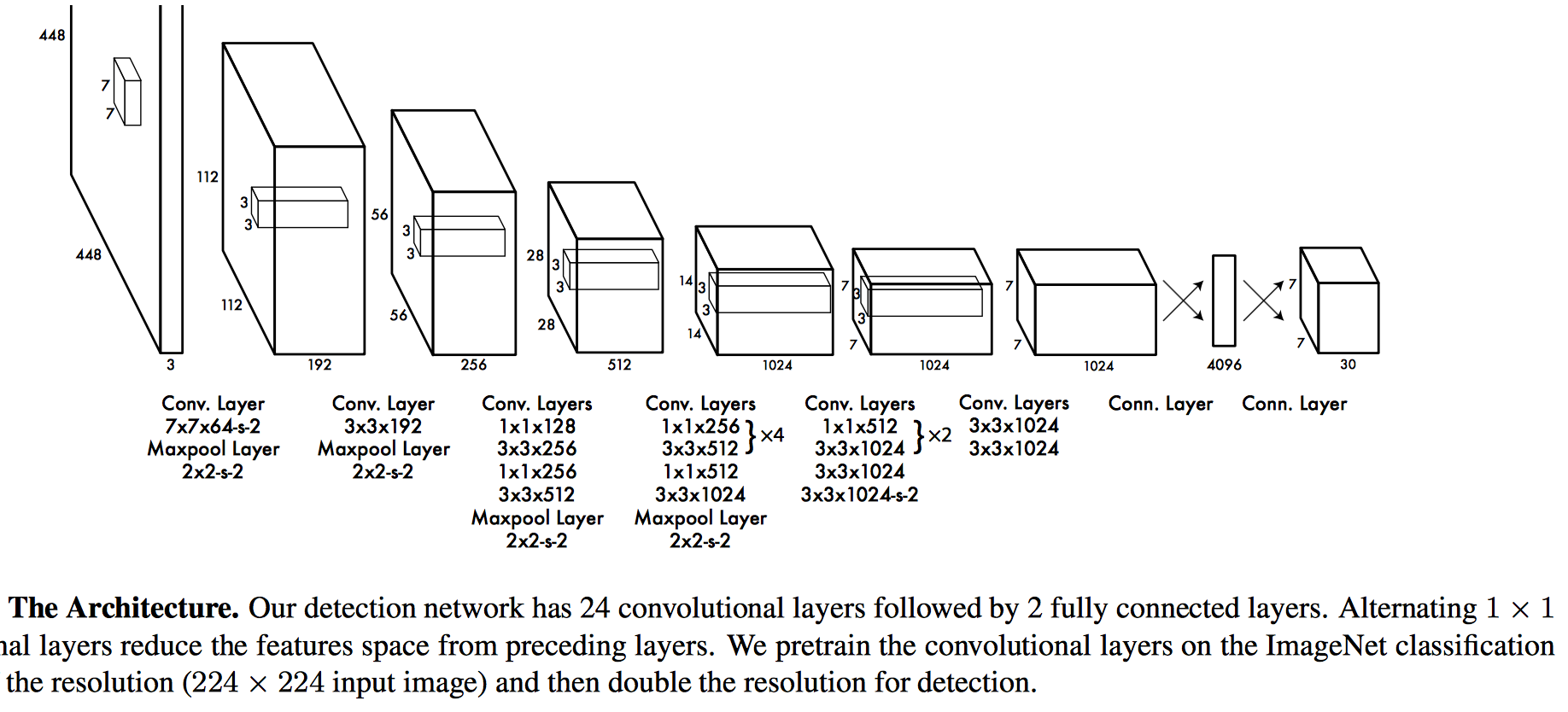
Convolutional layers are a special technique for dealing with image structure.
Sequences
In the supervised learning problem we had sets of sample/target pairs $(\mathbf x^{(k)}, y^{(k)})$.
Order of samples is assumed to not matter (in fact statistically it should not: "iid" assumption)
Training by using batches in random order actually appears to help.
A sequence is a dataset where the order is important information. E.g., text.
What other datasets are like this?
Sequence examples
Time series - often a single scalar value for each sample.
Text - a bunch of non-numeric characters.
GPS trajectories - a vector with coordinates, time-stamp, identity, other info
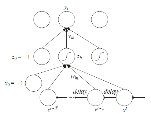
Time Delay Neural Networks
Waibel et al. 1989 - previous inputs are delayed in time so as to synchronize with the final input, and all are fed together as input to the system
Dealing with text data
We will focus on text as perhaps the most important kind of sequence data.
Consider supervised learning problem where we have a string of text for each sample, and class lables we want a to make a network to classify them into.
For example:
- Classify emails as spam or ham.
- Classify online posts as sarcastic or serious.
- Classify movie reviews as positive or negative
From Text to Numbers
Problem: text is not a vector of numbers. Artificial neural networks operate on numbers.
Idea zero: convert into ascii.
What are some problems with this approach?
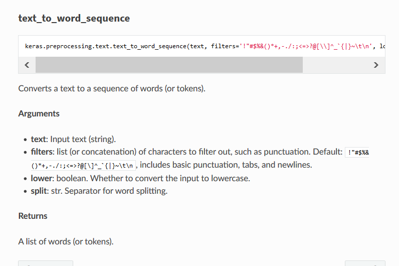
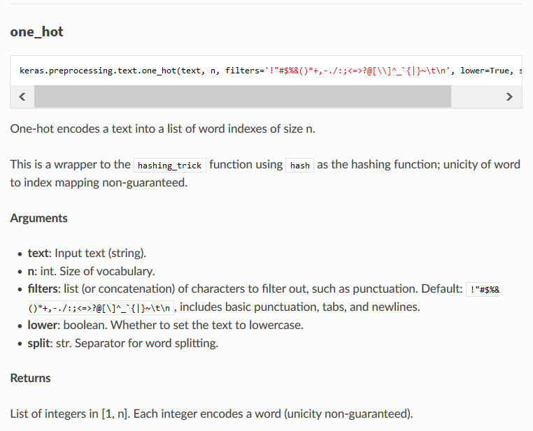
Tokens
First step is to break text string up into tokens, then convert each token into a number.
Possible choices for tokens: characters, words, sequences of n words ($n$-grams)
Most commonly, words are used.
Treat words as features - One-hot encoding
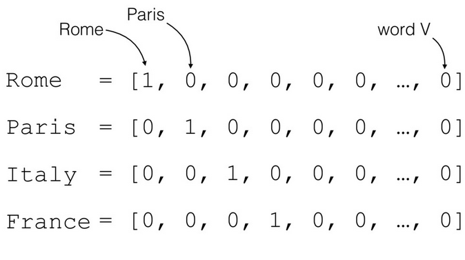
Have to choose which words to use. Can't use them all, some (a, and , the) less meaningful.
Position $k$ in vector means word $k$. Element $x_k = 1$ or 0 tells presence or absence of word $k$ in sample.
Bag-of-Words (BOW)
Convert a text string (like a document) into a vector of word frequencies by essentially summing up the one-hot encoded vectors for the words. Perhaps divide by total number of words.
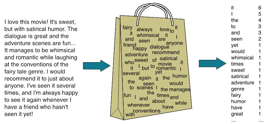
Basically get histogram for each documents to use as feature vectors. Becomes structured data.
Problem: order of words in sequence is lost. "A hates B" has same vector as "B hates A"
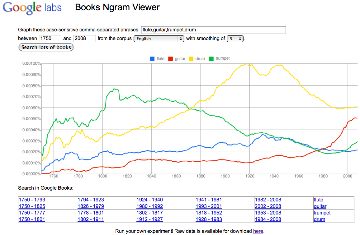
$n$-grams - Use little bit of order
Rather than encoding words, count short sequences of words of length $n$.
Generalize from words to "tokens", can choose to use characters, symbols, etc.
As $n$ increases can have many many more $n$-grams.
Keras does not have a function for this, but other packages do.
The bag-words-uses a special case of $n$-grams. What is it?
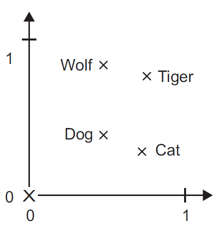
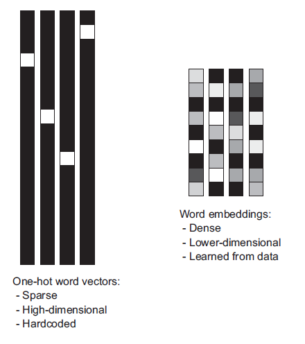
Word embeddings
One-hot encoding converts words (or $n$-grams) into orthogonal vectors $\mathbf e_k$ with a single "1" value and the rest zeros. Vectors for any two words are orthogonal. So to handle 50,000 words requires length-50,000 vectors.
Geometrically these are orthogonal vectors in 50,000-dimensional space. With every word vector equally-distant from every other.
Word embeddings try to squeeze these into a lower number of dimensions by putting "similar" words closer together, use real numbers (rather than only binary).
Embedding methods
- Principal component analysis & related methods applied to BOW data ~ Latent semantic indexing
- Shallow neural network layer - Embedding layer
- word2vec
Exercise: create a dense linear single-layer network (no activation function) with $N$ inputs and $m$ outputs, and write the output for a one-hot encoded input vector $\mathbf e_k$, as well as for a general input vector $\mathbf v$.
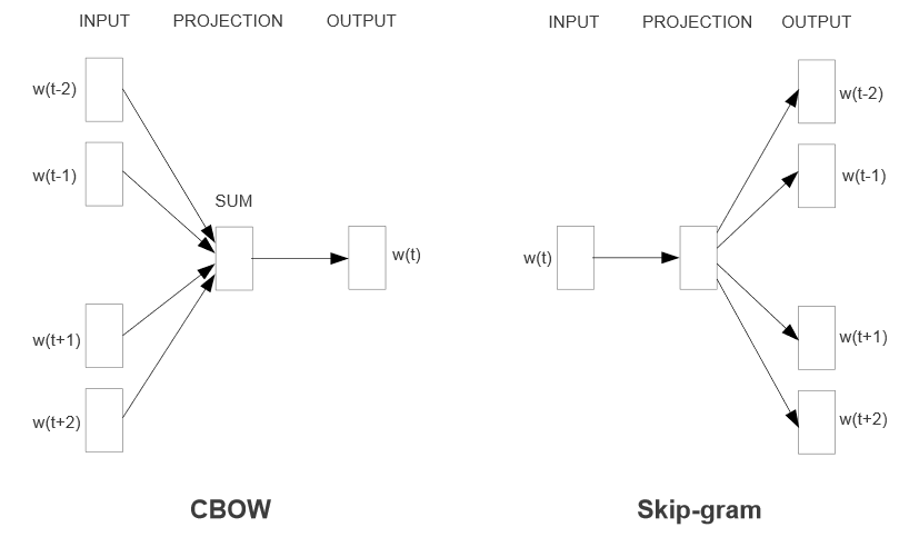
Word2Vec
Continuous bag of words - predict $k$th word using neighbors in a window
Skip-gram - predict neighboring words for $k$th word
The weights in the neural layer for prediction give the emedding vectors.
Can download and use result: https://code.google.com/archive/p/word2vec
GloVe
Dim reduction on matrix of co-occurence statistics.
Can download and use result: https://nlp.stanford.edu/projects/glove/
glove_dir = '/home/user01/Public/Data/Glove_embeddings'

embeddings_index = {}
f = open(os.path.join(glove_dir, 'glove.6B.100d.txt'))
for line in f:
    values = line.split()
    word = values[0]
    coefs = np.asarray(values[1:], dtype='float32')
    embeddings_index[word] = coefs
f.close()

print('Found %s word vectors.' % len(embeddings_index))
# make embedding matrix

embedding_dim = 100

embedding_matrix = np.zeros((max_words, embedding_dim))
for word, i in word_index.items():
    embedding_vector = embeddings_index.get(word)
    if i < max_words:
        if embedding_vector is not None:
            # Words not found in embedding index will be all-zeros.
            embedding_matrix[i] = embedding_vector
embedding_matrix.shape
Keras Embedding Layer
Literally download GloVe or word2vec and use .set_weights() to set it as weights
See Chollet Ch.6 for examples
from keras.models import Sequential
from keras.layers import Embedding, Flatten, Dense

model = Sequential()
model.add(Embedding(max_words, embedding_dim, input_length=maxlen))
model.add(Flatten())
model.add(Dense(32, activation='relu'))
model.add(Dense(1, activation='sigmoid'))
model.summary()
# Set embedding layer weights to GloVe matrix and freeze

model.layers[0].set_weights([embedding_matrix])
model.layers[0].trainable = False
Lab
Download embedding weights and compute cosine distances between similar words.
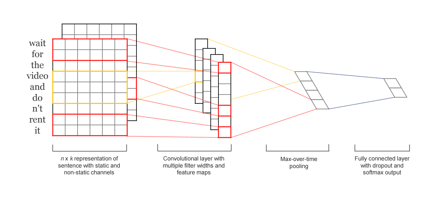
The next layer performs convolutions over the embedded word vectors using multiple filter sizes. For example, sliding over 3, 4 or 5 words at a time.
Next, the result of the convolutional layer is max-pooled into a long feature vector.
Create a classification prediction with a softmax layer.
from keras.datasets import imdb
from keras.preprocessing import sequence

max_features = 10000  # number of words to consider as features
max_len = 500  # cut texts after this number of words (among top max_features most common words)

print('Loading data...')
(x_train, y_train), (x_test, y_test) = imdb.load_data(num_words=max_features)
print(len(x_train), 'train sequences')
print(len(x_test), 'test sequences')

print('Pad sequences (samples x time)')
x_train = sequence.pad_sequences(x_train, maxlen=max_len)
x_test = sequence.pad_sequences(x_test, maxlen=max_len)
print('x_train shape:', x_train.shape)
print('x_test shape:', x_test.shape)
from keras.models import Sequential
from keras import layers
from keras.optimizers import RMSprop

model = Sequential()
model.add(layers.Embedding(max_features, 128, input_length=max_len))
model.add(layers.Conv1D(32, 7, activation='relu'))
model.add(layers.MaxPooling1D(5))
model.add(layers.Conv1D(32, 7, activation='relu'))
model.add(layers.GlobalMaxPooling1D())
model.add(layers.Dense(1))

model.summary()

model.compile(optimizer=RMSprop(lr=1e-4),
              loss='binary_crossentropy',
              metrics=['acc'])
history = model.fit(x_train, y_train,
                    epochs=10,
                    batch_size=128,
                    validation_split=0.2)
acc = history.history['acc']
val_acc = history.history['val_acc']
loss = history.history['loss']
val_loss = history.history['val_loss']

epochs = range(len(acc))

plt.plot(epochs, acc, 'bo', label='Training acc')
plt.plot(epochs, val_acc, 'b', label='Validation acc')
plt.title('Training and validation accuracy')
plt.legend()

plt.figure()

plt.plot(epochs, loss, 'bo', label='Training loss')
plt.plot(epochs, val_loss, 'b', label='Validation loss')
plt.title('Training and validation loss')
plt.legend();


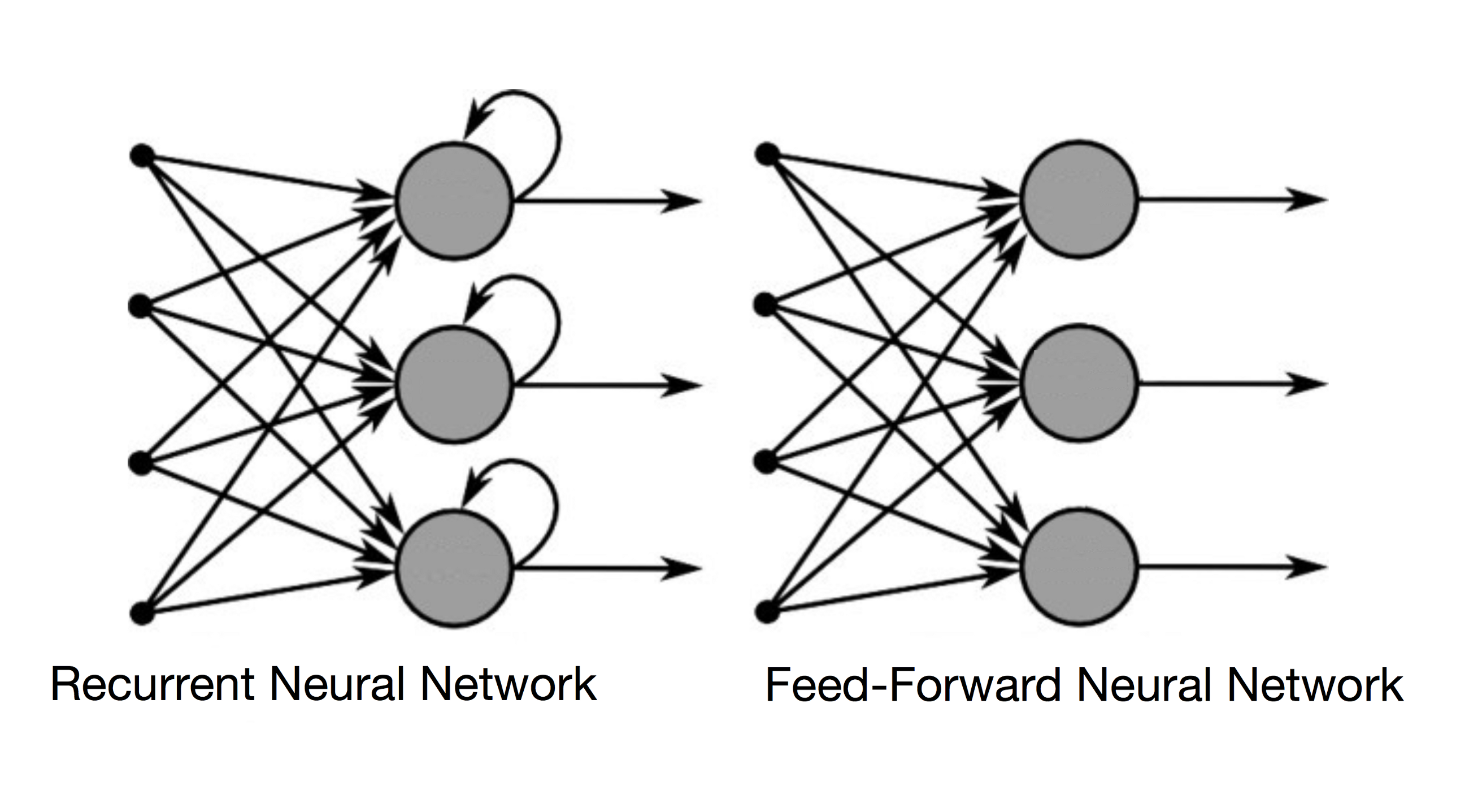
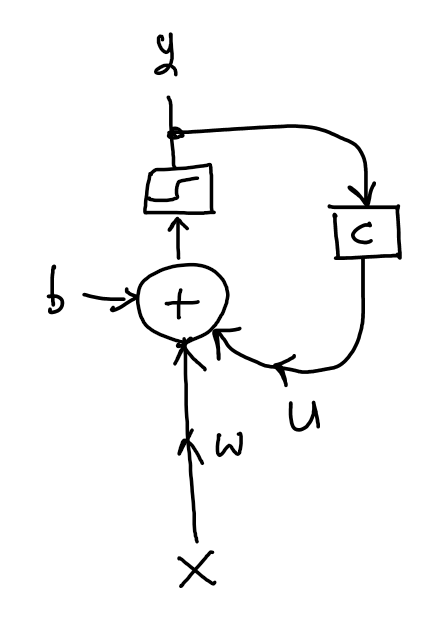
Recurrent Neural Networks
Thus far we have only considered network architectures where information flows in one direction from input layer to output layer.
If there are any connections taking information backwards, the network will contain a loop, and it is called a recurrent network.
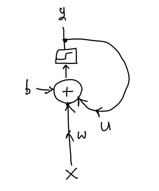
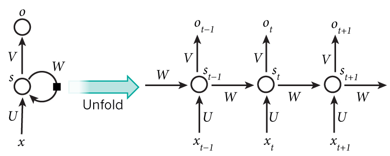
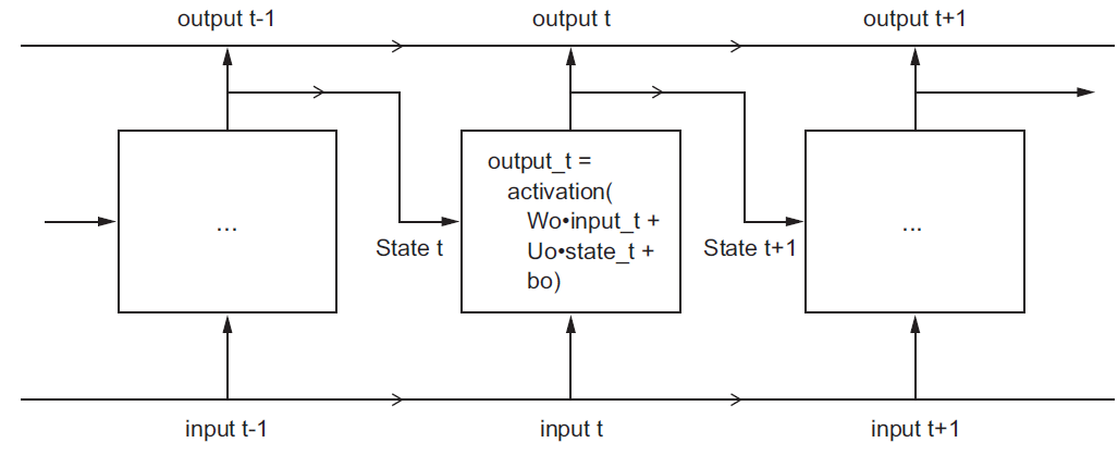
Unrolled RNN
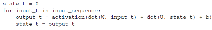
Write the sequence of inputs and outputs then consider as a single layer with a one-step calculation
Multiple neuron RNN Layer
Picture what it would look like to extend this to multiple neurons
- in series
- in parallel
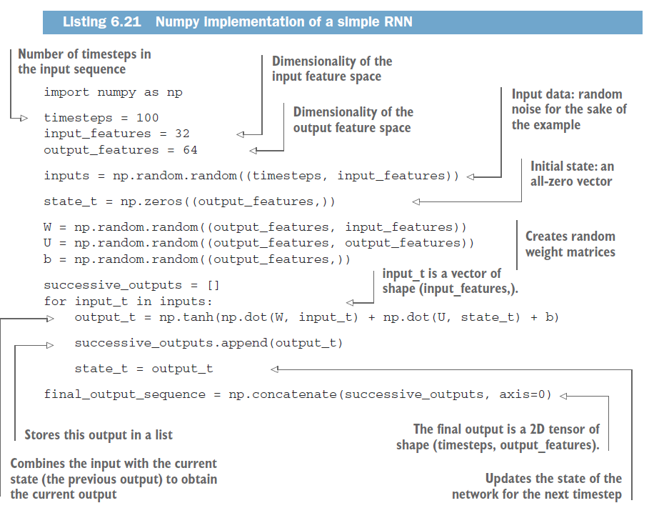
Keras Simple RNN
Process IMDB dataset
from keras.datasets import imdb
from keras import preprocessing

# Number of words to consider as features
max_features = 10000
# Cut texts after this number of words
# (among top max_features most common words)
maxlen = 20

# Load the data as lists of integers.
(x_train, y_train), (x_test, y_test) = imdb.load_data(num_words=max_features)

# This turns our lists of integers
# into a 2D integer tensor of shape `(samples, maxlen)`
x_train = preprocessing.sequence.pad_sequences(x_train, maxlen=maxlen)
x_test = preprocessing.sequence.pad_sequences(x_test, maxlen=maxlen)
Without RNN
from keras.models import Sequential
from keras.layers import Flatten, Dense

model = Sequential()
model.add(Embedding(10000, 8, input_length=maxlen))
model.add(Flatten())
model.add(Dense(1, activation='sigmoid'))
model.compile(optimizer='rmsprop', loss='binary_crossentropy', metrics=['acc'])
model.summary()

history = model.fit(x_train, y_train,
                    epochs=10,
                    batch_size=32,
                    validation_split=0.2)
RNN
from keras.layers import Dense
from keras.models import Sequential
from keras.layers import Embedding, SimpleRNN

model = Sequential()
model.add(Embedding(max_features, 32))
model.add(SimpleRNN(32))
model.add(Dense(1, activation='sigmoid'))

model.compile(optimizer='rmsprop', loss='binary_crossentropy', metrics=['acc'])
history = model.fit(input_train, y_train,
                    epochs=10,
                    batch_size=128,
                    validation_split=0.2)
Vanishing Gradient problem
As networks become very deep, the gradient terms in become approximately zero and the network cannot be trained.
Feedforward Solution: Residual connections a.k.a. skip connections - send output to later layers
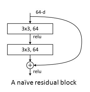
The gradient is larger via the shortcut.
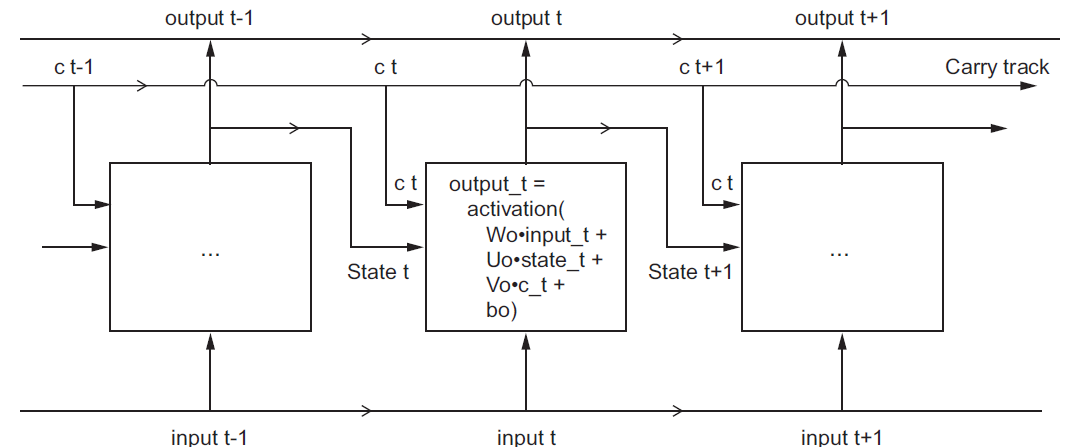
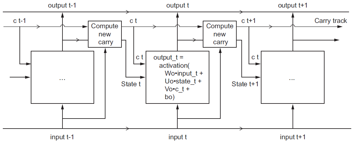
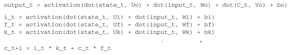
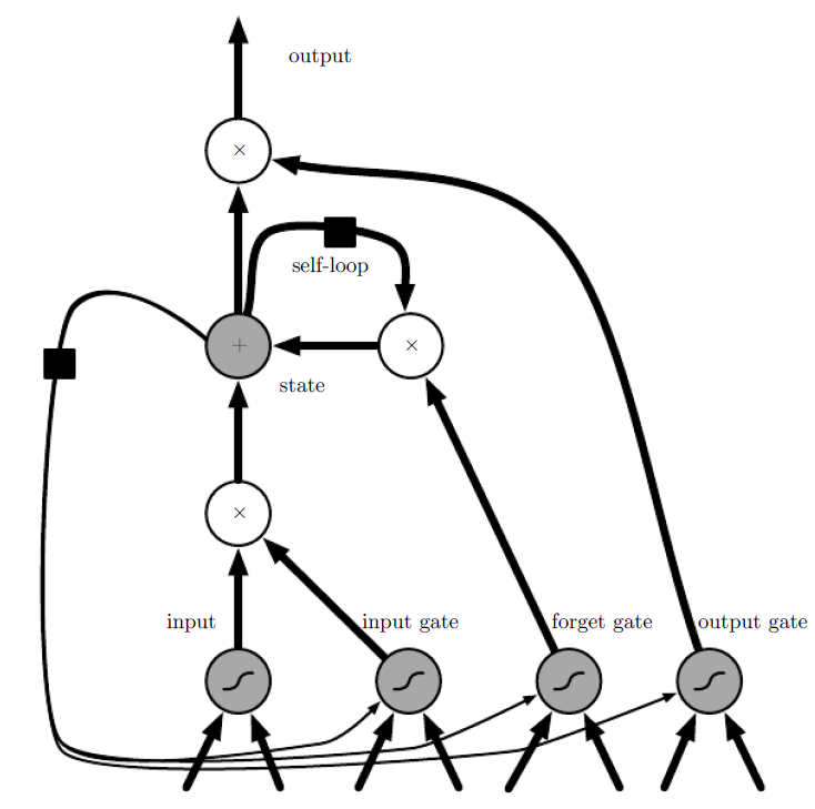
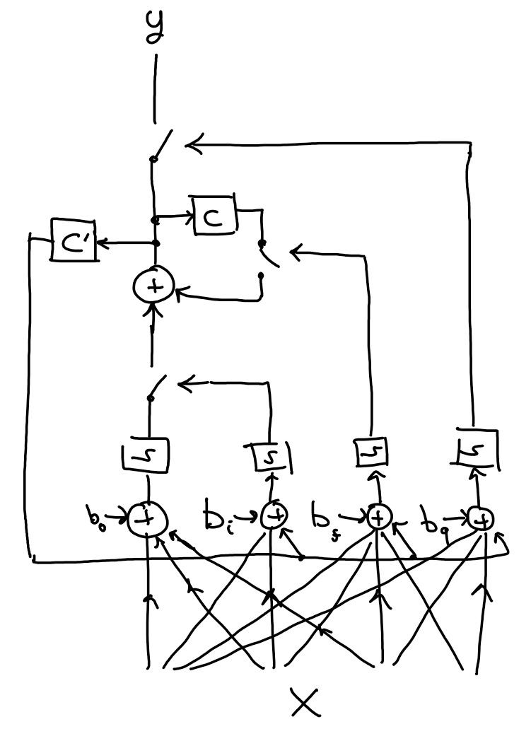
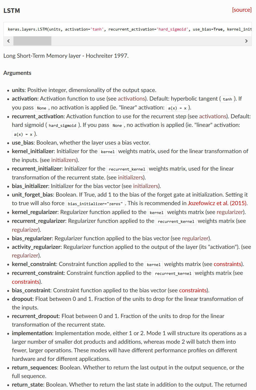
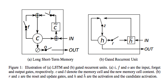
Long short-term memory networks (LSTM)
We can do the same idea in a feedback loop (unrolled here) ... "carry" signal
LSTM for IMDB
from keras.datasets import imdb
from keras.preprocessing import sequence

max_features = 10000  # number of words to consider as features
maxlen = 500  # cut texts after this number of words (among top max_features most common words)
batch_size = 32

print('Loading data...')
(input_train, y_train), (input_test, y_test) = imdb.load_data(num_words=max_features)
print(len(input_train), 'train sequences')
print(len(input_test), 'test sequences')

print('Pad sequences (samples x time)')
input_train = sequence.pad_sequences(input_train, maxlen=maxlen)
input_test = sequence.pad_sequences(input_test, maxlen=maxlen)
print('input_train shape:', input_train.shape)
print('input_test shape:', input_test.shape)
from keras.models import Sequential
from keras.layers import LSTM
from keras.layers import Dense
from keras.layers import Embedding

model = Sequential()
model.add(Embedding(max_features, 32))
model.add(LSTM(32))
model.add(Dense(1, activation='sigmoid'))

model.compile(optimizer='rmsprop',
              loss='binary_crossentropy',
              metrics=['acc'])
history = model.fit(input_train, y_train,
                    epochs=10,
                    batch_size=128,
                    validation_split=0.2)
Echo state networks
Another old idea. Build a randomly-connected network as a kind of noise generator.
Then add in put and output layers and train them to control the noise generation.
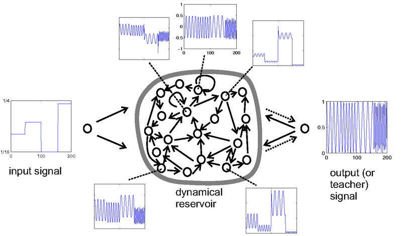
Basically a regression problem to find combination of internal signals to produce desired output.
- Liquid state machines
- Reservoir computing
Lab
Implement the CNN and LSTM for classifying the IMDB dataset.
Language Model
Given a sequence of tokens, we can train a network to give the probabilities of each possible token being next.
For text, this is sometimes called a language model, a statistical distribution over all possible text sequences.
$$ f(\mathbf x^{(k)},y^{(k)}) = P(y^{(k)}| \mathbf x^{(k)}) = P(\text{next word in sequence } | \text{ previous words}) $$How would you make the training dataset for this?
What activation function would you use?
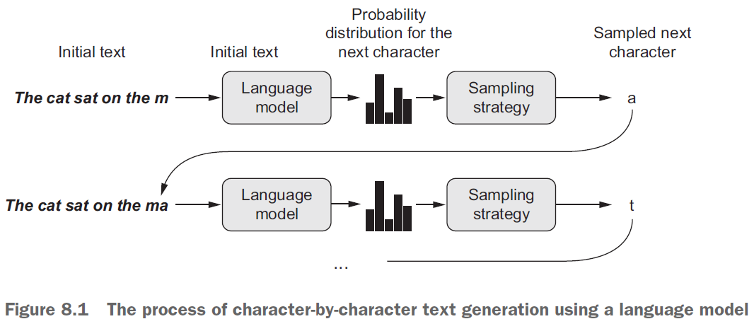
Text generation
Use characters as your tokens
Use the predicted character as part of the next input sequence to predict subsequent character
keep repeating this process
Temperature
A technique to change relative probabilities
Combine with a sampling strategy to pick classes randomly depending on $P(y| \mathbf x)$.
$$ P(y | \mathbf x) \rightarrow \exp\left( \frac{1}{T}\log(P(y| \mathbf x))\right) $$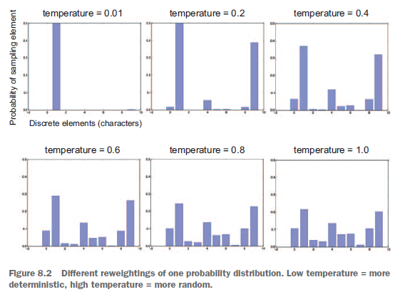
import numpy as np

path = keras.utils.get_file('nietzsche.txt',origin='https://s3.amazonaws.com/text-datasets/nietzsche.txt')
text = open(path).read().lower()
print('Corpus length:', len(text))
# Length of extracted character sequences
maxlen = 60

# We sample a new sequence every `step` characters
step = 3

# This holds our extracted sequences
sentences = []

# This holds the targets (the follow-up characters)
next_chars = []

for i in range(0, len(text) - maxlen, step):
    sentences.append(text[i: i + maxlen])
    next_chars.append(text[i + maxlen])
print('Number of sequences:', len(sentences))

# List of unique characters in the corpus
chars = sorted(list(set(text)))
print('Unique characters:', len(chars))
# Dictionary mapping unique characters to their index in `chars`
char_indices = dict((char, chars.index(char)) for char in chars)

# Next, one-hot encode the characters into binary arrays.
print('Vectorization...')
x = np.zeros((len(sentences), maxlen, len(chars)), dtype=np.bool)
y = np.zeros((len(sentences), len(chars)), dtype=np.bool)
for i, sentence in enumerate(sentences):
    for t, char in enumerate(sentence):
        x[i, t, char_indices[char]] = 1
    y[i, char_indices[next_chars[i]]] = 1