Hacking Math I
Spring 2020

Topic 5: Norms and Distances
This topic:
- Norms & Distances
- Simple distance-based classification
- Clustering
Reading:
- I2ALA Chapter 3 (Norms), Chapter 4 (Clustering)
- CTM Chapter 8 (The Inner Product)
- Strang I.11 (I.11 Norms of Vectors, Functions, and Matrices)
Metric
Basically, boil multiple numbers (vectors, matrices, time series,...) or entire functions down to a single number
Examples
- GDP of economy
- BMI (body-mass index)
- A statistic (mean, variance, ...)
- Vector norms...
Always can be critized as discarding important info, but need to use something
Euclidean Norm
$$ \|x\| = \sqrt{x_1^2+x_2^2+\dotsb+x_n^2} $$"Length" of a vector (as opposed to length of the data structure, i.e. number of dimensions)
Also known as $\|x\|_2$, the "two-norm"
Exercise: give Euclidean norm using dot products
Example
$$\left\Vert \begin{pmatrix}2 \\ -1\\2 \end{pmatrix}\right\Vert = ?$$Root-mean-square value (RMS)
$$ rms(x) = \sqrt{\frac{x_1^2+x_2^2+\dotsb+x_n^2}{n}} = \frac{1}{\sqrt{n}}\|x\| $$root(mean(square(x)))
Exercise: give Euclidean norm of sum of vectors $x+y$ in terms of dot products
(use result of previous exercise and work only with vectors)
Chebychev Inequality
If $x$ is a length-$n$ vector with $k$ entries satisfying $|x_i|\ge a$ for some constant $a>0$, then
$$\frac{k}{n} \le \left( \frac{rms(x)}{a}\right)^2$$Basically tells how much elements can deviate from the rms
Derive by noting that $\Vert x\Vert^2 \ge ka^2$
Motivation for other types of norms
Consider the list of data for different "dimensions", for one person, product, etc.
Does it make sense to compute Euclidean distance to tell us how "big" the vector is?
Norms
A norm is a vector "length". Often denoted generally as $\Vert \mathbf x \Vert$.
Properties
- Non-negativity: $\Vert \mathbf x \Vert \geq 0$
- Zero upon equality: $\Vert \mathbf x \Vert = 0 \iff \mathbf x = \mathbf 0$
- Absolute scalability: $\Vert \alpha \mathbf x \Vert = |\alpha| \Vert \mathbf x \Vert$ for scalar $\alpha$
- Triangle Inequality: $\Vert \mathbf x + \mathbf z\Vert \leq \Vert \mathbf x\Vert + \Vert \mathbf z\Vert$
$p$-Norms
For any $n$-dimensional real or complex vector. i.e. $x \in \mathbb{R}^n \text{ or } \mathbb{C}^n$
$$ \|x\|_p = \left(|x_1|^p+|x_2|^p+\dotsb+|x_n|^p\right)^{\frac{1}{p}} $$$$ \|x\|_p = \begin{pmatrix}\sum_{i=1}^n{|x_i|^p} \end{pmatrix}^{\frac{1}{p}} $$Consider the norms we have looked at. What is $p$?
Famous "norms"
- $\ell_2$ norm
- $\ell_1$ norm
- $\ell_\infty$ norm
- $\ell_p$ norm
- "$\ell_0$" norm
Note we often lazily write these as e.g. "L2" norm, though mathematicians will complain because that mas a slightly different meaning already.
Exercise: Wite out the $p$-norms for a vector $x$ for $p$ = 1,2,0,$\infty$... $ \|x\|_p = \begin{pmatrix}\sum_{i=1}^n{|x_i|^p} \end{pmatrix}^{\frac{1}{p}} $
Exercise: test the conditions for each
import numpy as np

v = [1,3,1,4]

for p in range(1,10):
    print(p,np.power(sum(np.power(np.abs(np.array(v)),p)),1/p))
Exercise
What are the norms of $\vec{a} = \begin{bmatrix}1\\3\\1\\-4\end{bmatrix}$ and $\vec{b} = \begin{bmatrix}2\\0\\1\\-2\end{bmatrix}$?
"Norm balls"
The Set $\{x | \Vert x \Vert_p \le 1 \}$, $ \|x\|_p = \begin{pmatrix}\sum_{i=1}^n{|x_i|^p} \end{pmatrix}^{\frac{1}{p}} $
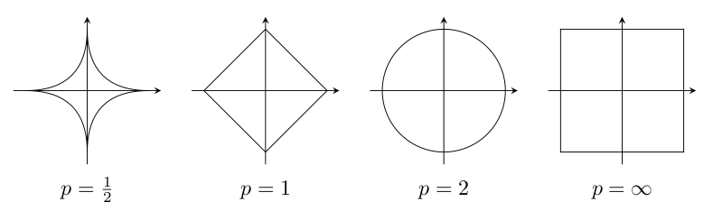
Note how $\Vert x \Vert_a \le \Vert x \Vert_b$ if $a\ge b$
Norms, Inner products, and angles
Inner product = length squared
$$v \cdot v = v^T v = \| v \|_2$$Angle $\theta$ between two vectors
$$v \cdot w = v^T w = \| v \|_2\| w \|_2 \cos\theta$$Cauchy-Schwartz Inequality $v^T w \le \| v \|\| w \|$
Triangle Inequality
$$\| v + w \| \le \| v \|+\| w \|$$Derive by noting that $\| v + w \|^2 = \|v\|^2 + v^Tw + \|w\|^2$ then use Cauchy-Schwartz and complete square
$S$-norm
For any symmetric positive definite matrix $S$
$$\| v \|_S = v^T S v$$$S$ inner product
$$<v,w>_S = v^T S w$$Minkowski metric
Proposed by Lorentz for 4-dimensional spacetime, $v = (x,y,z,t)^T$, $c$ is speed of light
$$\| v\|^2_M = x^2+y^2+z^2-ct^2$$Is it a true norm?
II. Distances
Euclidean distance between two vectors $a$ and $b$ in $\mathbb{R}^{n}$:
$$d(\mathbf a,\mathbf b) = \sqrt{\sum_{i=1}^{n}(b_i-a_i)^2}$$Again this may not make sense for various vectors. Many alternatives...
Norm versus Distance
What is the relationship?
Distance properties
A distance metic $d(\mathbf x,\mathbf y)$ must satisfy four particular conditions to be considered a metric:
- Non-negativity: $d(\mathbf x,\mathbf y) \geq 0$
- Zero upon equality: $d(\mathbf x,\mathbf y) = 0 \iff \mathbf x = \mathbf y$
- Commutativity of arguments: $d(\mathbf x,\mathbf y) = d(\mathbf y,\mathbf x)$
- Triangle Inequality: $d(\mathbf x,\mathbf z) \leq d(\mathbf x,\mathbf y) + d(\mathbf y,\mathbf z)$
Exercise
Write the Euclidean distance between two points entirely in terms of dot products.
What does this tell you about using dot products to compare vector similarity?
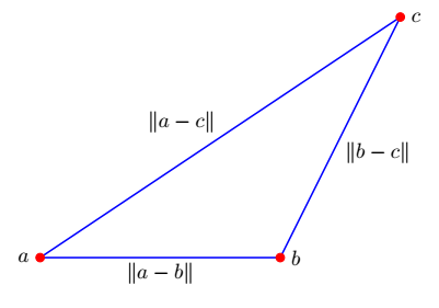
Triangle Inequality
$\Vert \mathbf x + \mathbf z\Vert \leq \Vert \mathbf x\Vert + \Vert \mathbf z\Vert$
$d(\mathbf a,\mathbf c) \leq d(\mathbf a,\mathbf b) + d(\mathbf b,\mathbf c)$
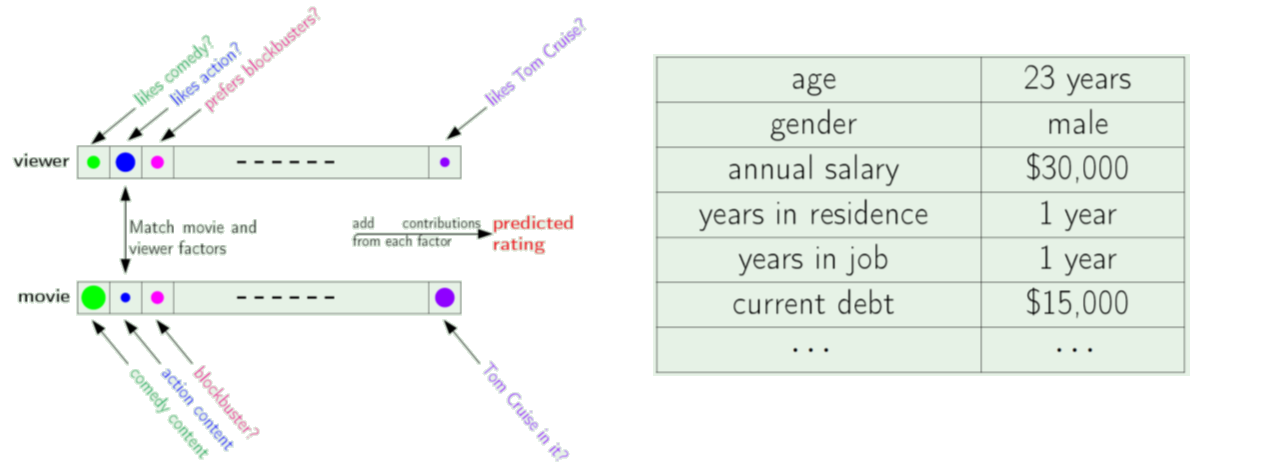
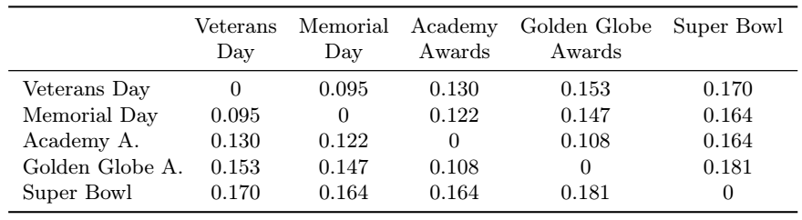
Application: feature distances
Recommender syatem based on most similar customers to movie properties
Question: what are the units of the distance here?
Application: rms prediction error
Time series prediction (stocks or temperature) compared to truth in retrospect
Manhattan or "Taxicab" Distance, also "Rectilinear distance"
Measures the relationships between points at right angles, meaning that we sum the absolute value of the difference in vector coordinates.
This metric is sensitive to rotation.
$$d_{M}(a,b) = \sum_{i=1}^{n}|b_i-a_i|$$...consider
- Non-negativity: $d(\mathbf x,\mathbf y) \geq 0$
- Zero upon equality: $d(\mathbf x,\mathbf y) = 0 \iff \mathbf x = \mathbf y$
- Commutativity of arguments: $d(\mathbf x,\mathbf y) = d(\mathbf y,\mathbf x)$
- Triangle Inequality: $d(\mathbf x,\mathbf z) \leq d(\mathbf x,\mathbf y) + d(\mathbf y,\mathbf z)$
Exercise
Does it fulfill the 4 conditions?
Chebyschev Distance
The Chebyschev distance or sometimes the $L^{\infty}$ metric, between two vectors is simply the the greatest of their differences along any coordinate dimension:
$$d_{\infty}(\mathbf a,\mathbf b) = \max_{i}{|(b_i-a_i)|}$$...consider
- Non-negativity: $d(\mathbf x,\mathbf y) \geq 0$
- Zero upon equality: $d(\mathbf x,\mathbf y) = 0 \iff \mathbf x = \mathbf y$
- Commutativity of arguments: $d(\mathbf x,\mathbf y) = d(\mathbf y,\mathbf x)$
- Triangle Inequality: $d(\mathbf x,\mathbf z) \leq d(\mathbf x,\mathbf y) + d(\mathbf y,\mathbf z)$
Cosine Distance
High school geometry: $\mathbf a \cdot \mathbf b = \|\mathbf a\|_2\|\mathbf b\|_2 \cos\theta$
Only depends on angle between the vectors
$$d_{\cos}(\mathbf a,\mathbf b) = 1-\frac{\mathbf a \cdot \mathbf b}{\|\mathbf a\|\|\mathbf b\|} = 1 - \cos\theta$$Not a true distance metric. which propery fails to hold? (easy to guess at based on geometry)
Exercise
Implement the metrics manually and compute distances between:
$ \begin{bmatrix} 1 \\ 2 \\ 3 \\ 4 \end{bmatrix}$ and $ \begin{bmatrix} 5 \\ 6 \\ 7 \\ 8 \end{bmatrix}$
III. Matrix Norms
Matrix norms: motivation
Same goal as with vector norms: determining if matrices are small or large, or if two matrices are similar or different
Numerical mathematics example: you use 32-bit precision numbers to compute the inverse of a matrix. How different from the true inverse is your numerical calculation? Suppose you used 64-bit precision instead? (FYI the errors can be much larger than $2^{-32}$ or $2^{-64}$)
# https://www.mathworks.com/help/matlab/ref/cond.html

A1 = [[4.1, 2.8],
      [9.7, 6.6]]
print(np.linalg.inv(A1))

A2 = [[4.1,    2.8  ],
      [9.671,  6.608]]
print(np.linalg.inv(A2))
Matrix norms
The set of matrices can be viewed as a vector space (contains origin, closed under addition and scalar multiplication), hence we can define a norm analogously for lengths and distances
Conditions of a norm
- $\|A\| \ge 0$, only equal if $A$ is zero matrix
- $\|cA\| = |c| \|A\|$
- $\|AB\| \le \|A\|\|B\|$ ...new rule for matrix norms
Matrix norms: Froenius Norm
- Frobenius Norm $\Vert A \Vert_F = \sqrt{\sigma_1^2+..+\sigma_r^2} = \sum_{ij}A_{ij}^2$
Exercise: Compute $\|AB\|_F$
Orthogonal matrix
Doesn't change L2 norm of vector or Frobenius norm matrix
$$\Vert Qx\Vert_2 = \Vert x\Vert_2$$$$\Vert QB\Vert_F = \Vert B\Vert_F$$Matrix norms from vector norms via vectorization
Just "vectorize" the matrix then apply a vector norm.
What do you get if you use the L2 vector norm for this?
Matrix norms from vector norms via matrix-vector product
Given a vector norm $\|v\|_\psi$, we can always make a matrix norm as follows
\begin{align} \|A\|_\psi &= \max_{x \ne 0}\dfrac{\Vert Ax \Vert_\psi}{\Vert x\Vert_\psi} \\ &= \max_{x \ne 0, \Vert x\Vert_\psi = 1}\Vert Ax \Vert_\psi \end{align}What does that give?
- $\ell_2$ $\rightarrow$ $\|A\|_2 = \sigma_1$, largest singular value of $A$
- $\ell_1$ $\rightarrow$ $\|A\|_1 = \max_{column_i}\|column_i\|_1 $, largest absolute column sum
- $\ell_\infty$ $\rightarrow$ $\|A\|_\infty = \max_{row_i}\|row_i\|_1 $, largest absolute row sum
Connections
$$\|A\|_\infty = \|A^T\|_1$$$$\|A\|_2^2 \le \|A\|_1 \|A\|_\infty$$Spectral and related norms
- Spectral Norm $\Vert A \Vert_2 = \max \dfrac{\Vert Ax \Vert}{\Vert x\Vert} = \sigma_1$, a.k.a. $\ell_2$ norm
- Frobenius Norm $\Vert A \Vert_F = \sqrt{\sigma_1^2+..+\sigma_r^2} = \sum_{ij}A_{ij}^2$
- Nuclear norm $\Vert A \Vert_N = \sigma_1+..+\sigma_r$, a.k.a. trace norm
Exercise: compute norms for $I$
Spectral Radius
$$|\lambda|_{\max} = \max_i |\lambda_i|$$Useful metric that does not fulfill properties of norm
For every posible (true) norm, we have $\|A\| \ge |\lambda|_{\max}$
Useful fact: if $|\lambda|_{\max} <1$, $\|A^k\| \rightarrow 0$ for large $k$
Can you explain why this happens?
"Medical norm"
$$|||A|||_\infty = \max_{i,j}|A_{i,j}|$$Not a true matrix norm unless scaled properly also
See Strang problem I.11 #12.
Condition number
Quantifies how much output changes relative to a change in input.
Low condition number - good - "well conditioned"
- a small chance in inputs due to noise or numerical precision only causes a small change in output
Huge condition number - bad - "ill conditioned"
- even a tiny change in inputs can cause a drastic change in outputs. result unreliable
Condition number for solving linear system $Ax=b$
- View the function as $x = A^{-1}b$ where input = $b$ and output = $x$.
- Relative fractional error
Taking the max over $b$ and $\delta$ gives
\begin{align} C &= \max_{b,\delta} \dfrac{\|A^{-1}\delta\|}{\|A^{-1}b\|}\dfrac{\|b\|}{\|\delta\|} \\ &= \left(\max_{\delta}\dfrac{\|A^{-1}\delta\|}{\|\delta\|}\right) \left(\max_{b}\dfrac{\|b\|}{\|A^{-1}b\|} \right) \\ &= \|A^{-1}\|\|A\| \end{align}First term is just definition of matrix norm. For second term, plug in $b = Ax$ and get norm definition also, noting that max will be the same optimizing over $x$ or over $Ax$ since $A$ is full-rank.
"Matrix Condition number"
Usually means condition number with L2 norm
Recall $\|A\|_2 = \sigma_\max(A)$
$$C \equiv \|A^{-1}\|_2\|A\|_2 = \dfrac{\sigma_\max(A)}{\sigma_\min(A)}$$Suppose a matrix is singular? (what does this mean?)
- what are its singular values?
- what is its condition number?
# https://www.mathworks.com/help/matlab/ref/cond.html

A1 = [[4.1, 2.8],
      [9.7, 6.6]]
print(np.linalg.inv(A1))

A2 = [[4.1,    2.8  ],
      [9.671,  6.608]]
print(np.linalg.inv(A2))
print(np.linalg.cond(A1),np.linalg.cond(A2))
v1 = np.array([1.,2.])

A = np.array([v1,2.*v1])

print(A)
print('rank =',np.linalg.matrix_rank(A))
An = A + 1e-10*np.random.rand(2,2)
print('rank =',np.linalg.matrix_rank(An))
print('cond =',np.linalg.cond(An))
Exercise
Test the prior matrices when solving a linear system $Ax=b$ and adding a small perturbation to $b$
Change the matrix to make it wekk conditioned and repeat,
IV. Distance-based Classification
Lab: simple classification with distances
Load and investigate the IRIS dataset from scikit.
Imagine we flower measurements for one of the flowers but don't know the flower type. We want to classify its type by finding the flower of known type which is most similar.
Do this by taking each flower and computing a distance metric between its measurements and that of every other flower. Take the type of the "nearest" flower as your estimate of the flower type.
Compute the accuracy of this technique based on how many flowers are classified correctly in this way.
Try using different distance metrics to compare flowers. Which makes most sense?
from sklearn import datasets
iris = datasets.load_iris()

dir(iris)
(iris.data, iris.target)
iris.data[52]
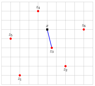
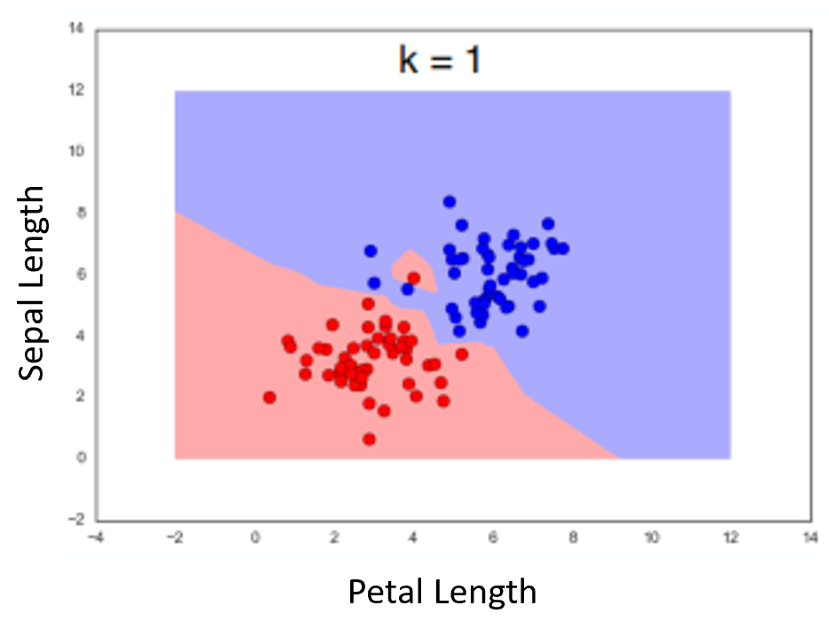
The "1-Nearest-Neighbor" Algorithm
Example using two features. Dots represent the measurements for the flowers in the dataset. Color of background is class of nearest neighbor (as if the point was the measurements for an unknown flower we were classifying)
Hamming or "Rook" Distance
The hamming distance can be used to compare nearly anything to anything else.
Defined as the number of differences in characters between two strings of equal length, ie:
$$d_{hamming}('bear', 'beat') = 1$$$$d_{hamming}('cat', 'cog') = 2$$$$d_{hamming}('01101010', '01011011') = 3$$Edit distance
Similar to hamming distance, but also includes insertions and deletions, and so can compare strings of any length to each other.
$$d_{edit}('lead', 'gold') = 4$$$$d_{edit}('monkey', 'monk') = 2$$$$d_{edit}('lucas', 'mallori') = 8$$- A kind of approximate matching method.
- Must use dynamic programming or memoization for efficiency
V. Clustering
Dimensionality Reduction
Describing data with less information
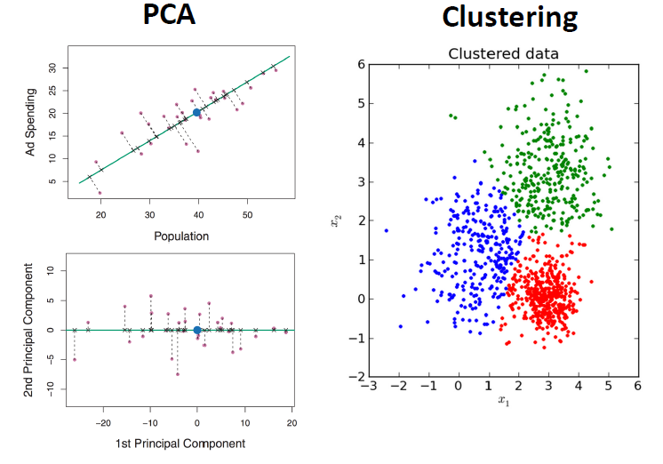
How are PCA and Clustering leading to less information? Consider a dataset.
What are the benefits?
Clustering References
https://en.wikipedia.org/wiki/K-means_clustering
https://en.wikipedia.org/wiki/K-means%2B%2B - kmeans++
https://www.youtube.com/watch?v=IuRb3y8qKX4 - video with visualization of training progress
https://www.youtube.com/watch?v=cWSnFaSjgBU - more on visualization
http://scikit-learn.org/stable/modules/generated/sklearn.cluster.KMeans.html
Marketing Motivation
You want to make a certain number of products for a large population of customers. We know a number of features describing each of the customers, and are able to target a product to a certain customer profile.
E.g.: different customers prefer cars which are fast, or get good gas mileage, or are cheap, or are luxurious and presigious (i.e., expensive), or are big, or are little, etc. And in various combinations.
The customers vary widely so we wish to make k products which cover as closely as possible what as many as possible customers would like.
The better you can do this, the better your products will sell.
K-means clustering
- K clusters, centers are the means of cluster members.
- Each sample belongs to the cluster who's mean is nearest.
- Iteratively recompute membership and means (greedy optimization)
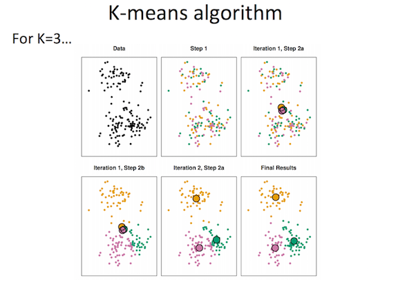
K-means algorithm
- Assign a number from 1 to K to each of N data points randomly
- While cluster assignments keep changing:
- For each of K clusters:
- Calculate cluster centroid
- For each of N points:
- Assign point to centroid it is closest to
- For each of K clusters:
Consider the possible ways to vary details in this method? How many clusters? How calculate distance?
k-Means as Greedy Optimization
The sum of all distances between members of a cluster gives a total length (a squared length can be viewed as a measure of "energy").
Within-Cluster-Variation: $WCV(C_k) = \dfrac{1}{|C_k|}\sum_{i, j \in C_k}d(x_{i}-x_{j})$, where $d(x_{i}-x_{j})$ is a distance metric of your choice.
k-means tries to minimize the net lengths over all clusters.
If you plotted this for each iteration, what would the plot look like?
Lab
Implement k-means clustering algorithm using scikit on IRIS, MNIST datasets.
Compute the net WCV for various options.
Look at result and WCV with different initializations.
Try varying the metric used in the clustering.
Vary k and plot WCV versus k.
Scikit hints
Hyperparameter k is input into constructor as usual
Clustering done with a stereotpyical "Fit()" method
Results (cluster centers, cluster label for each point) stuck in attributes, as usual. ".inertia_" ~ WCV)
Variants of k-Means
It's often possible by being creative to come up with ways to define a distance for unusual data types.
For example: comparing books with distance defined as (inverse) number of common words. Both contan "the", "soufle", france", etc.
But it still may not make sense to average the data. Why is this a problem? What might be done instead?