Hacking Math I

Spring 2020

Topic 6: Statistics

This topic:

1. Single-variable Statistics
2. Preprocessing data
3. Multidimensional statistics

Reading: *

I. Single-variable Statistics

Statistics: Describing data and Populations

Not just the data we have, but presuming our numbers apply to a population we sampled from:

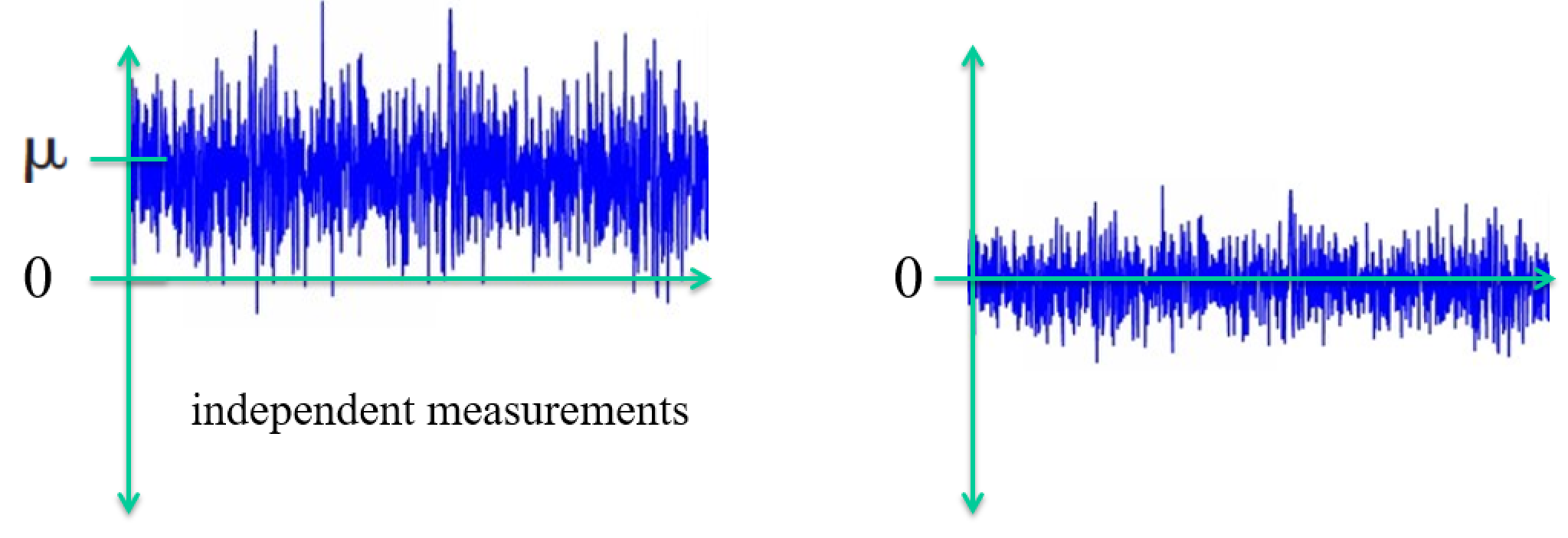
Example: we want to know the average age of college students in the US, so we ask the members of this class and take the average.

What's the sample here?

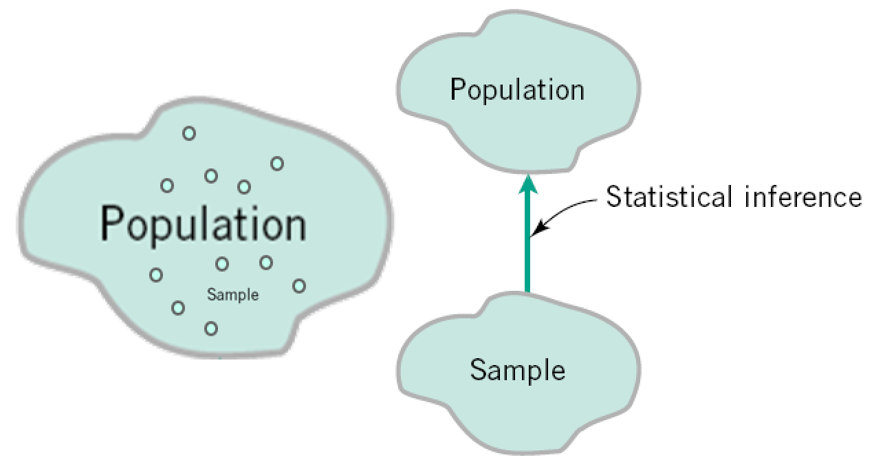
Note: "sample" can refer to individual measurements or the entire set depending on field.

Randomness

Random variable $X$ - a variable whose measured value can change from one replicate of an experiment to another. E.g., the unknown coin flip result.

"Range of $X$" = values it can take, a.k.a. outcomes. E.g., $\{HEADS, TAILS\}$.

New kind of notation $P(X=x)$ aka $Prob(X=x)$ is probability that the random variable $X$ will take the value of $x$ in an experiment.

E.g., $P(\text{coin flip result} = HEADS)$

$P(\text{"event"})$ can be very abstract, such as $P(X\le 5)$ or $P(X\le 5, X\ge 2)$.

How does relate to the statisticians' "sample"?

Probability

A probability $P(\text{"event"})$ is a number between 0 and 1 representing how likely it is that an event will occur.

Probabilities can be:

1. Frequentist: $\dfrac{\text{number of times event occurs}}{\text{number of opportunities for event to occur}}$

2. Subjective: represents degree of belief that an event will occur

E.g. I think there's an 80% chance it will be sunny today $\rightarrow$ P(sunny) = 0.80

The rules for manipulating probabilities are the same, regardless how we interpret probabilities.

New Concepts

1. Probability $P(X=x)$

2. Distribution - a theoretical version of a histogram:

1. Expectation $E(\cdot )$ - a theoretical version of a mean: $ \bar{x} \rightarrow E(x) $

Discrete Distribution - Probability Mass Function $f(x_i) = P(X = x_i)$

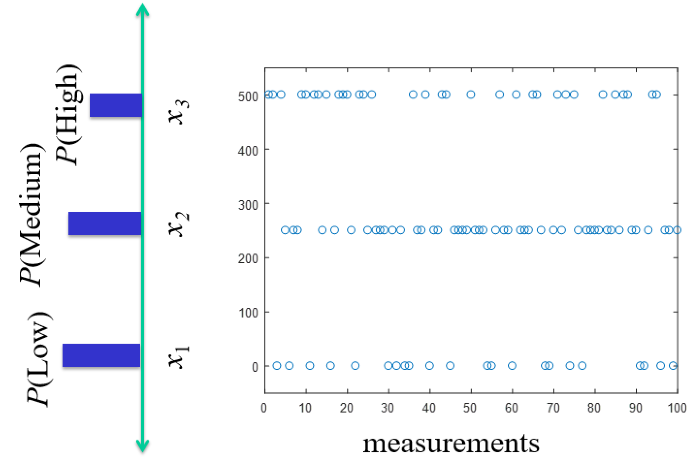
Remember $f(x_i)$ aren't values we measure, they're probabilities for values we measure (or relative frequencies).

** So scale histogram by total to make numbers relative for distribution.

Exercise

We flip a coin 100 times and get 60 heads and 40 tails.

1. What is (apparently) $P(X=HEADS)$ and $P(X=TAILS)$?
2. What might the distribution look like?

Statistics functions: Expectation, Mean & Variance

For a statistical population, when $x_i$ are independent samples: \begin{align} \text{Population mean} &= \mu = \frac{\sum_{i=1}^N x_i}{N} \\ \text{Population variance} &= \sigma^2 = \frac{\sum_{i=1}^N (x_i - \mu)^2}{N} \\ \end{align}

For a random variable $X$, for which all possible values are $x_1$, $x_2$,... $x_N$: \begin{align} \text{Mean} &= \mu = E(X) = \sum_{i=1}^N x_i f(x_i) \\ \text{Variance} &= \sigma^2 = V(X) = E(X-\mu^2) = \sum_{i=1}^N x_i^2 f(x_i) - \mu^2 \\ \end{align}

Theoretical way to accomplish the same thing by adding them up smarter.

Three-sided example $x_1=0,x_2=1,x_3=2$

Samples are in the list: [1, 0, 2, 0, 1, 0, 1, 1, 2, 0, 1]

So what are the relative frequencies of $x_1$, $x_2$, and $x_3$?

What is the sample mean?

What is $E[X]$ using formula?

Three-sided example $x_1=0,x_2=1,x_3=2$

Samples are: 1, 0, 2, 0, 1, 0, 1, 1, 2, 0, 1

\begin{align} \text{Population mean} &= \mu = \frac{\sum_{i=1}^N x_i}{N} \\ &= \frac{1}{11}(1 + 0 + 2 + 0 + 1 + 0 + 1 + 1 + 2 + 0 + 1)1 \text{, for a population of 11 } \\ &= \frac{1}{11}(0+0+0+0) + \frac{1}{11}(1+1+1+1+1) + \frac{1}{11}(2+2)\\ &= \frac{1}{11} 4\times 0 + \frac{1}{11} 5\times 1 + \frac{1}{11} 2 \times 2 \\ &= \frac{4}{11} \times 0 + \frac{5}{11} \times 1 + \frac{2}{11} \times 2 \\ &\approx f(x_1) x_1 + f(x_2) x_2 + f(x_3) x_3 \text{ the relative frequency} \end{align}\begin{align} \text{Mean, a.k.a. Expected value} &= \mu = E(X) = \sum_{i=1}^N x_i f(x_i) \\ \end{align}

Statistics with vectors

Assume the samples are in a vector $v$

1. Compute the mean using linear algebra
2. for the vector $v$ with its mean removed

Continuous Distributions - Probability Density Function $f(x) = P(X = x)$

Essentially just the continuous limit. Sums $\rightarrow$ integrals.

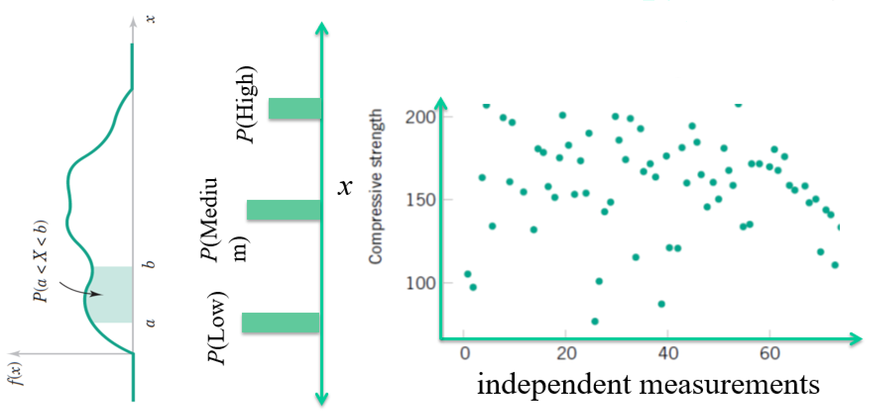
Where is the list of samples (e.g. the vector) here?

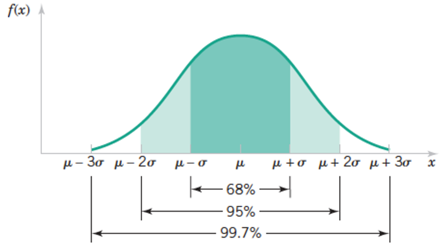
The Normal Distribution

• Most widely-used model for the distribution of a random variable
• Central limit theorem (good approximation to most situations)
• Also known as Gaussian distribution

$$ f(x) = \frac{1}{\sqrt{2\pi}\sigma} e^{\frac{-(x-\mu)^2}{2\sigma^2}} \text{ for } -\infty < x < \infty $$\begin{align} E(X) &= \mu \\ V(X) &= \sigma^2 \end{align}

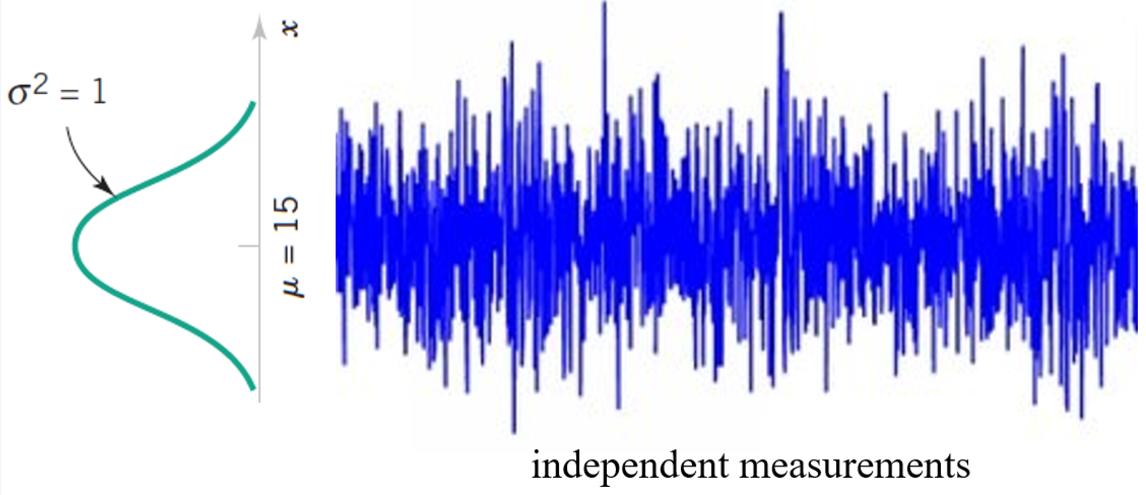
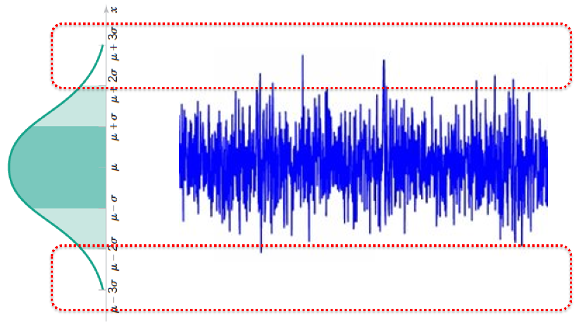
The Normal Distribution $X \sim N(\mu, \sigma)$

$$ f(x) = \frac{1}{\sqrt{2\pi}\sigma} e^{\frac{-(x-\mu)^2}{2\sigma^2}} \text{ for } -\infty < x < \infty $$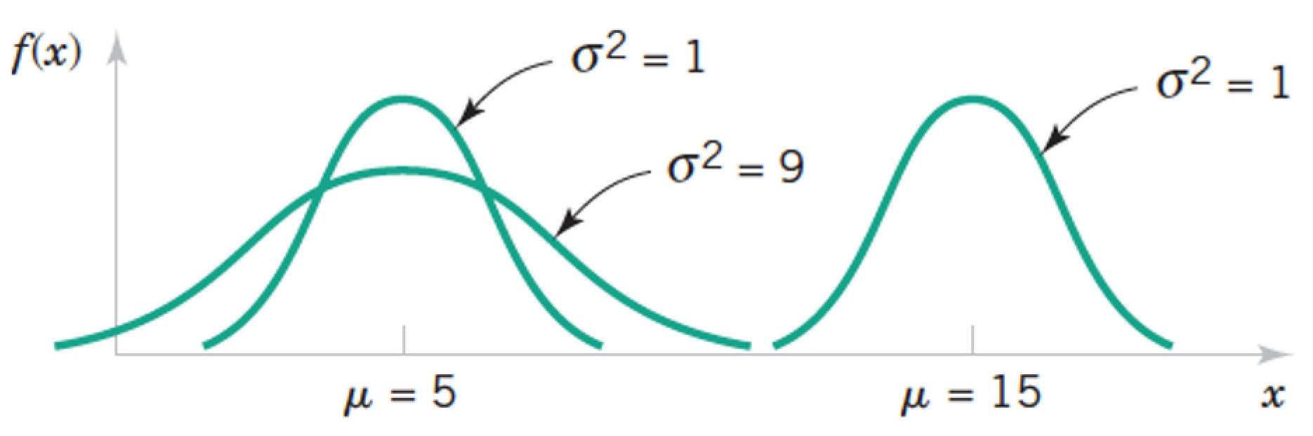

The Normal Distribution $X \sim N(\mu, \sigma)$

The Normal Distribution $X \sim N(\mu, \sigma)$

Which Gaussian describes which plot trace?

import numpy as np
from matplotlib import pyplot as plt

def univariate_normal(x, mean, var):
    return ((1. / np.sqrt(2 * np.pi * var)) * np.exp(-(x - mean)**2 / (2 * var)))

x = np.linspace(-5,5,1000)
plt.plot(x,univariate_normal(x,1,2));
plt.show()

Exercise

Generate normal random samples with mean of 1 and variance of 1

Plot histogram versus the theoretical distribution

Try different numbers of samples

Tails of the Normal Distribution $X \sim N(\mu, \sigma)$

Tails of the Normal Distribution $X \sim N(\mu, \sigma)$

The Standard Normal Distribution $Z$

• If $X$ is a normal r.v. with $E(X) = \mu$ and $V(X) = \sigma^2$

$$ Z = \frac{X-\mu}{\sigma} $$

• $Z$ is a normal r.v. with $E(X) = 0$ and $V(X) = 1$

• "Standardizing" the data

Standardizing data has two tasks

$$ Z = \frac{X-\mu}{\sigma} $$

1. Remove the mean
2. scale by the standard deviation

"de-meaned" vector

$$x - avg(x)$$

How is it done with dot products

Standard Deviation

$$ std(x) = \sqrt{\dfrac{(x_1 - avg(x))^2+...+(x_n - avg(x))^2}{n}} $$

Exercise

1. Load a dataset from sklearn and compute mean and variance of a column

2. Standardize the column

3. Now compute mean and variance of the result

Statistics

Consider the relation between norms and simple statistical quantities

\begin{align} \text{Population mean} &= \mu = \frac{\sum_{i=1}^N x_i}{N} \\ \text{Sample mean} &= \bar{x} = \frac{\sum_{i=1}^n x_i}{n} \\ \text{Population variance} &= \sigma^2 = \frac{\sum_{i=1}^N (x_i - \mu)^2}{N} \\ \text{Sample variance} &= s^2 = \frac{\sum_{i=1}^n (x_i - \bar{x})^2}{n - 1} = \frac{\sum_{i=1}^n x_i^2 - \frac{1}{n}(\sum_{i=1}^n x_i)^2}{n - 1} \\ \text{Standard deviation} &= \sqrt{\text{Variance}} \end{align}

Exercise:

Assume you have a vector containing samples. Write the following in terms of norms and dot products:

1. mean
2. variance
3. Correlation coefficient
4. Covariance

So what does this tell you about comparing things using distances versus dot products versus statistics?

II. Preprocessing Data

Preprocessing

We can now perform a variety of methods for preprocessing data.

Suppose we put our data (such as the Iris data) into vectors, one for each flower measurement ("feature").

We could:

• Remove the means (commonly done in many methods)
• Scale by 1/norm (often called "normalizing")

Standardizing a vector

1. remove the mean
2. Scale by 1/(standard deviation)

What is the mean and variance now?

"Standard" comes from standard normal distribution.

Lab: Normalizing data

Standardize the columns of the Iris dataset using linear algebra.

Test it worked by computing the mean and norm of each column.

III. Multidimensional Statistics

Correlation(s)

\begin{align} \text{Variance } s^2 &= \frac{\sum_{i=1}^n (x_i - \bar{x})^2}{n - 1} = \frac{\sum_{i=1}^n x_i^2 - \frac{1}{n}(\sum_{i=1}^n x_i)^2}{n - 1} \\ \text{Standard deviation} &= \sqrt{\text{Variance}} \end{align}\begin{align} \text{Correlation Coefficient } r &= \frac{ \sum_{i=1}^n (x_i - \bar{x})(y_i - \bar{y})}{\sqrt{\sum_{i=1}^n(x_i - \bar{x})^2}\sqrt{\sum_{i=1}^n(y_i - \bar{y})^2}} = \frac{S_{xy}}{\sqrt{S_{xx} S_{yy}}} \\ %\text{''Corrected Correlation''} % &= S_{xy} = \sum_{i=1}^n (x_i - \bar{x})(y_i - \bar{y}) % = \sum_{i=1}^n x_i y_i - \frac{1}{n}(\sum_{i=1}^n x_i)(\sum_{i=1}^n y_i) \\ \text{Covariance} &= S_{xy} = \frac{1}{n-1}\sum_{i=1}^n (x_i - \bar{x})(y_i - \bar{y}) % = \sum_{i=1}^n x_i y_i - \frac{1}{n}(\sum_{i=1}^n x_i)(\sum_{i=1}^n y_i) \end{align}

Look kind of familiar? Relate to variance.

Review: Joint Distributions

Scatter diagram versus joint probability density.

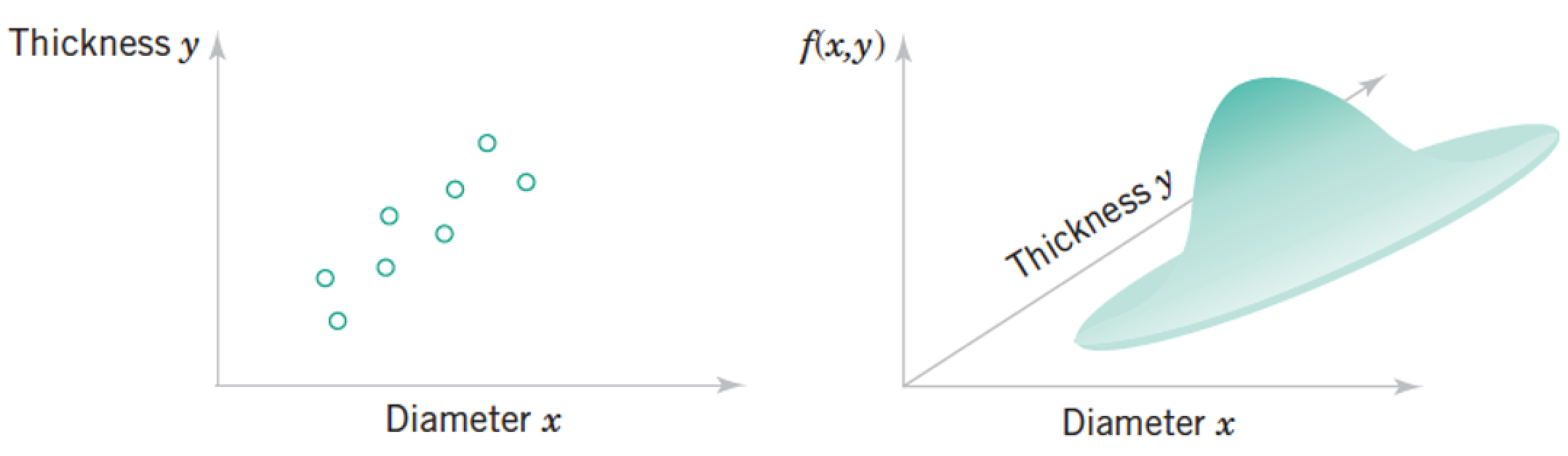
Each "sample" as a list of features, which we model as a vector of random variables, $ \mathbf x = \begin{pmatrix} Diameter \ Thickness

\end{pmatrix}

\begin{pmatrix} x_1 \\ \vdots \\ x_n \\ \end{pmatrix}

$

Each point in the distribution is simultanous probability of all the features taking the particular vector of numbers at the point.

Multivariate Data - describing relationships

"Multivariate" dataset ~ a matrix with samples for rows and features for columns. Each column (a.k.a. feature) is also known as a variable.

Just focusing on two variables for the moment, say column1 = $x$, and column2 = $y$.

Examples

How would you describe these relationships?

Correlation(s)

\begin{align} \text{Variance} &= s^2 = \frac{\sum_{i=1}^n (x_i - \bar{x})^2}{n - 1} = \frac{\sum_{i=1}^n x_i^2 - \frac{1}{n}(\sum_{i=1}^n x_i)^2}{n - 1} \\ \text{Standard deviation} &= \sqrt{\text{Variance}} \end{align}\begin{align} \text{Correlation Coefficient} &= r = \frac{ \sum_{i=1}^n (x_i - \bar{x})(y_i - \bar{y})}{\sqrt{\sum_{i=1}^n(x_i - \bar{x})^2}\sqrt{\sum_{i=1}^n(y_i - \bar{y})^2}} = \frac{S_{xy}}{\sqrt{S_{xx} S_{yy}}} \\ %\text{''Corrected Correlation''} % &= S_{xy} = \sum_{i=1}^n (x_i - \bar{x})(y_i - \bar{y}) % = \sum_{i=1}^n x_i y_i - \frac{1}{n}(\sum_{i=1}^n x_i)(\sum_{i=1}^n y_i) \\ \text{Covariance} &= S_{xy} = \frac{1}{n-1}\sum_{i=1}^n (x_i - \bar{x})(y_i - \bar{y}) % = \sum_{i=1}^n x_i y_i - \frac{1}{n}(\sum_{i=1}^n x_i)(\sum_{i=1}^n y_i) \end{align}

Look kind of familiar? Relate to variance. Note $"Cov(x,x)" = S_{xx}= \sigma_x^2$.

Questions

• What are $S_{xx}$ and $S_{yy}$ also called?

• Can you relate the covariance to a distance metric?

Exercises

\begin{align} \text{Correlation Coefficient} &= r = \frac{ \sum_{i=1}^n (x_i - \bar{x})(y_i - \bar{y})}{\sqrt{\sum_{i=1}^n(x_i - \bar{x})^2}\sqrt{\sum_{i=1}^n(x_i - \bar{x})^2}} = \frac{S_{xy}}{\sqrt{S_{xx} S_{yy}}} \end{align}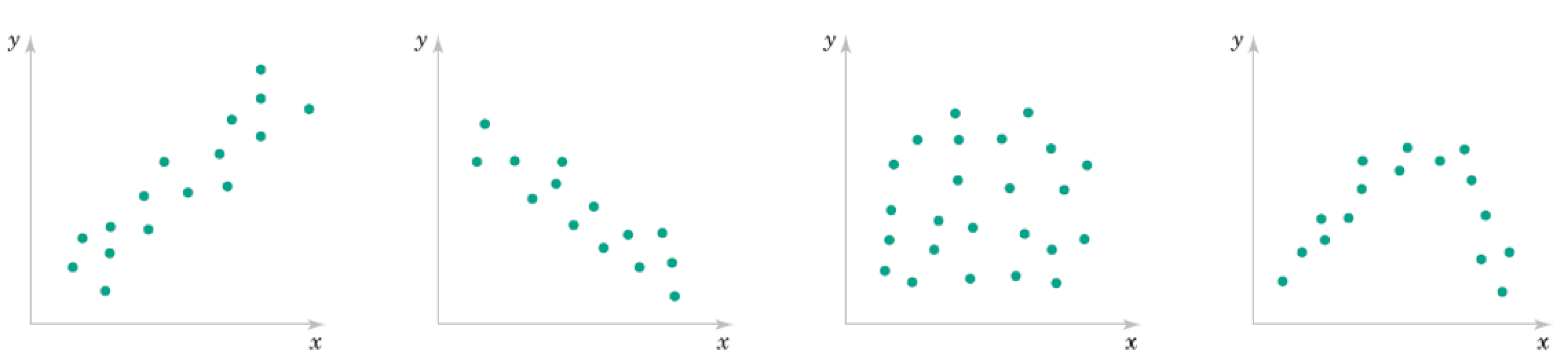

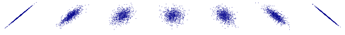
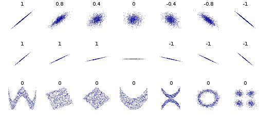
Roughly what are the correlation coefficients here?

Harder Exercises I

Roughly what are the correlation coefficients here?

Harder Exercises II

Roughly what are the correlation coefficients here?

Correlation Qualitative Behavior

1. What does magnitude tell you about the relationship?
2. What does sign tell you about the relationship?
3. Would you expect the Covariance to be similar?

And of course, Correlation does not prove Causation

Most important statistics fact ever?

Tricky Exercise

Consider a $m \times 3$ matrix $\mathbf A$ with columns $\mathbf x, \mathbf y$, and $\mathbf z$ (each a vector of data).

Suppose we standardize the three columns to make $\bar{\mathbf A}$.

What are the elements of $\bar{\mathbf A}^T \bar{\mathbf A}$?

Multivariate Gaussian (for $n$ dimensions)

$$ f(\mathbf x) = \frac{1}{ \sqrt{2 \pi^n |\boldsymbol\Sigma|}} \exp \left(- \frac{1}{2} (\mathbf x - \boldsymbol \mu)^T \boldsymbol\Sigma^{-1} (\mathbf x - \boldsymbol \mu) \right) \text{, for } \mathbf x \in R^n $$

• Mean vector as centroid of distribution
• Covariance matrix describes spread - correlations between variables $\Sigma_{ij} = S_{\mathbf x_i \mathbf x_j}$

\begin{align} \text{Correlation Coefficient} &= r = \frac{ \sum_{i=1}^n (x_i - \bar{x})(y_i - \bar{y})}{\sqrt{\sum_{i=1}^n(x_i - \bar{x})^2}\sqrt{\sum_{i=1}^n(y_i - \bar{y})^2}} = \frac{S_{xy}}{\sqrt{S_{xx} S_{yy}}} \\ %\text{''Corrected Correlation''} % &= S_{xy} = \sum_{i=1}^n (x_i - \bar{x})(y_i - \bar{y}) % = \sum_{i=1}^n x_i y_i - \frac{1}{n}(\sum_{i=1}^n x_i)(\sum_{i=1}^n y_i) \\ \text{Covariance} &= S_{xy} = \frac{1}{n-1}\sum_{i=1}^n (x_i - \bar{x})(y_i - \bar{y}) % = \sum_{i=1}^n x_i y_i - \frac{1}{n}(\sum_{i=1}^n x_i)(\sum_{i=1}^n y_i) \end{align}

...Terminology note...

In general terms, covariance is a kind of metric for correlation.

Formal definition of correlation (i.e. Pearson) differs from covariance only in scaling, so that it ranges between $\pm 1$ rather than some max and min.

I will tend to use them interchangeably, where correlation means the more intuitive concept and covariance the formal matrix we compute (or its elements).

def multivariate_normal(x, n, mean, cov):
    return (1./(np.sqrt((2*np.pi)**n * np.linalg.det(cov))) * np.exp(-1/2*(x - mean).T@np.linalg.inv(cov)@(x - mean)))


mean = np.array([35,70])
cov = 100*np.array([[1,.5],[.5,1]])
pic = np.zeros((100,100))
for x1 in np.arange(0,100):
    for x2 in np.arange(0,100):
        x = [x1,x2]
        pic[x1,x2] = multivariate_normal(x, 2, mean, cov)
        
plt.contour(pic);

cov

array([[100.,  50.],
       [ 50., 100.]])

np.linalg.inv(cov)

array([[ 0.01333333, -0.00666667],
       [-0.00666667,  0.01333333]])

Exercise: independence of random variables

$$P(x_1,x_2) = P(x_1)P(x_2)$$

What does the mean for a multivariate Gaussian distribution?

Using Covariance matrix as a Weighted adjacency matrix

Recall we could equivalently use the (first) eigenvectors of $\mathbf L_{rw}$ or the (last) eigenvectors of $\mathbf W$.

Consider the choice $\mathbf W = \mathbf C = \mathbf X \mathbf X^T$

What is $W_{ij}$ in terms of data samples?

How do the eigenvectors of $\mathbf W$ relate to singular vectors of $\mathbf X$?

Multivariate Gaussians as Networks

Recall use of covariance matrix as way to define network, covariances for similarities between variables

In this case, can view entire network as a description of a multivariate Gaussian distribution

• nodes represent random variables
• edges represent dependencies between random variables, nonzero off-diagonal terms in the covariance matrix

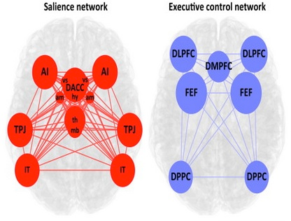
Example: brain networks inferred by measuring pairwise correlations between different regions

Note the sample covariance matrix is only an estimate of the true covariance between random variables. And in general the covariance between samples of data will never be zero. So we may choose to threshold small values in the covariance matrix. Or perhaps use more sophisticated means to find a sparse covariance matrix given data. The problem of finding better estimates is called covariance estimation.

Also note that it doesn't make too much sense to say that a pair of random variables are dependent on a third variable, but somehow independent of each other. Everything will tend to look connected to everything else.

Covariance Estimation

The problem of estimating a valid covariance matrix from data

Methods we know: computing sample covariances.

Network-inspired idea: compute sample covariance and set small values to zero for making s spase network.

Problem #1: will these estimates be invertible? (as we need to describe the Gaussian)

Problem with using Correlations for network edges

Pretty much everything will have some degree of correlation with everything else.

Consider a sequence of words with the bigram assumption. Distant words are still correlated even though they are conditionally independent.

Lab

1. Generate N Gaussian random numbers and compute mean and std and plot histograms, for N=10,100,1000.

2. Load IRIS dataset and compute pairwise correlations between features.

3. Now standardize each feature and give scatter plot for pairs of columns with highest pairwise correlation. Also give scatter plot for the pair of columns with lowest pairwise correlation.